Robotic stippling: Finding optimal sequences
or: Abusing lab equipment v3
In part 1, and part 2 of this series, I looked at overengineering 'making dots on a piece of paper' by using multiple robots. So far, I was not too concerned with finding an optimal solution, but rather with finding a solution that works well for one (in part 1) or two (in part 2) robots. Now, I want to look at how big the difference between an optimized solution, and the greedy solutions I produced so far is.
In previous posts, I looked at finding poses for robot arms to make dots, sorting the poses, and then finding paths for one robot in part 1, and for two robots in part 2. Even though this is part 3, I am not going to look at extending our approach to three robots (for now).
Instead, I am going back to only a single robot arm, and will compare the previous approach of generating a single dot-making-pose and greedily ordering the poses to generating multiple poses, and ordering them more optimally.I do not yet want to claim the optimal path, since I am still making a few approximations that impact the optimality along the way.
Problem setting
I am still assuming that I am getting a set of dots (2d coordinates) as input and want to output a path in joint-space of the robot that makes those dots onto the paper. I am not taking dynamics of the robot into account, i.e. I am planning geometrically only. This simplification is a valid approximation, since we have a good low lever controller, that (if we are not operating at very high speeds or with high loads) can track the path that a geometric planner produces well.
Compared to part 1, we are trying to optimize the path a little bit, instead of only looking for a reasonably good path. That is, our objective is time-optimality: Ideally, we want to find the path that makes all the dots the fastest. However, as alluded to before, finding the optimal path maps roughly to the traveling salesman problem, which is notoriously hard.
Additionally, since every dot can be made from various poses, we have multiple groups of poses which need to be visited exactly once. This is called the “Traveling Salesman Problem in Neighbourhoods”.
Instead of actually computing the time-optimal path between all poses, we use the infinity norm as distance metric between poses.I.e. the distance between two poses is the maximum absolute difference between all its elements This represents the time it takes to get from pose 1 to pose 2 fairly well, since a typical controller would steer each joint of the robot arm seprarately, i.e. the time it takes to get from pose 1 to pose 2 is the maximum time one of the joints takes.
Prior research for the traveling salesman problem with neighbourhoods are e.g. [1], [2], [3], or the two following here, which are concerned with robotics versions of the travelling salesman problem: [4] [5].
The problem we are tackling here is an ‘easy’ version of the two robotics papers above, since we do not have any obstacles in the environment which may make our path planning harder. The goal we have is then finding a good sequence of poses given a set of poses for each dot, i.e. finding both the sequence, and finding the right pose.
‘Solving’ the TSP for a single pose
First, we implement a ‘proper’ TSP algorithm for the single-pose case. Even though we likely have little enough poses to being able to find the exact solution, exhaustive search does not scale well, and we are thus skipping that approach directly.
We are implementing two approximation algorithms in addition to the purely greedy approach from before:
- Greedy with longer lookahead
- Simulated annealing
In both cases, I run the resulting path through an algorithm that tries to improve the result that we got. Here, I do that by locally reversing subtours and checking if that leads to a better result.
Simulated annealing is a well discussed approach for the TSP, and thus, I’ll only link to some other resources here: 1, 2. For me, an exponential cooling schedule worked well, and the transformations of the current solution I used were ‘swapping poses’ and ‘randomly reversing subtours’.
‘Solving’ the TSP for a neighbourhood
Finding a solution to the TSP with neighbourhoods can be done in various ways. However, as for the standard TSP, we are not getting the optimal solution here, but rather an approximation, since solving it is computationally not tractable.
We are going to look at a baseline of simply being greedy and simulated annealing for the neighbourhoods. I originally also planned to implement a greedy version with lookahead, but already did the experiments for a single pose, and noticed that the simulated annealing approach was much better, or said differently: The lookahead sometimes made the solution worse.
Simulated annealing for TSP with neighbourhoods: is close to the normal simulated annealing, except that we also need to include an operation that swaps poses. Thus, the transformations we use are the two from above, and swapping poses for a randomly chosen dot.
Comparison & Results
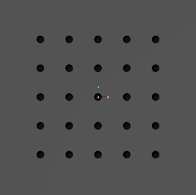
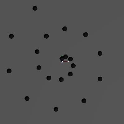
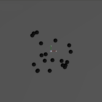
To compare the planners we produced above, we need a few testcases. We largely reuse things we have used before: a grid, a set of random points, a spiral, and part of our labs logo.
The methods I have implemented are summarized in the table below along with the pathlength of the method for each test. I marked the best result for both single-pose, and neighbourhoods italic, and the best overall in bold.
| Method | Grid | Random | Spiral | Logo | |
|---|---|---|---|---|---|
| Single pose | Greedy | 5.83 | 2.392 | 3.72 | 0.85 |
| Greedy with lookahead l=2 | 5.794 | 2.465 | 3.78 | 0.845 | |
| Simulated annealing | 5.681 | 2.389 | 3.589 | 0.838 | |
| Neighbourhood | Greedy | 4.915 | 1.474 | 4.347 | 0.841 |
| Simulated annealing | 4.732 | 1.390 | 4.241 | 0.807 |
And here is how the dots in the grid are ordered by the methods.
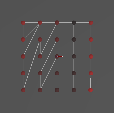
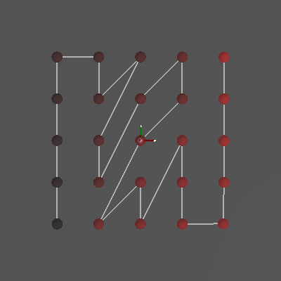
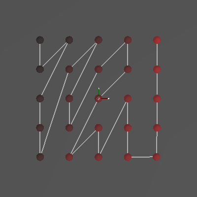
The ordering above does not seem like it makes a lot of sense from an optimality standpoint. What we are interested in is the time the robot takes for a given path. Since each joint typically has its own maximum velocity, the time each path segment takes is limited by the longest distance a single joint has to cover. We can compute the maximum velocity of each joint during the path segment, and then scale all the velocities such that the largest velocity in the segment reaches the maximum velocity. From this, we can then compute the total time each path segment would take, and thus compute the total time the robot takes for the path.
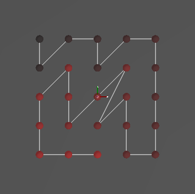
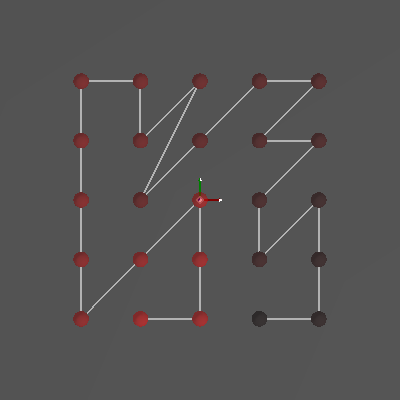
Finally, here is a side-by-side comparison of the greedy with sets and the TSP with a set of poses.
With times 1.902 and 1.422 (reload the page to restart the gifs at the same time).
Takeaway
I once more want to point out that the order of the dots does not necessarily seem to make sense as the ‘best’ path. The path we should get here should correspond to the shortest/best path in joint space of the robot, and thus be reasonlably close to a time-optimal path.
It came as a surprise to me that the methods with a longer lookahead do not necessarily outperform the simple methods. This likely has two reasons:
- We always perform a polishing step after we found the initial path, and some of the solutions that we obtain with a shorter lookahead might turn out better.
- The other reason is that the greedy methods are suboptimal, and it might simply be the case that a method with a longer lookahead is locally better, but turns out worse overall. (I.e. the longer lookahead digs itself into a deeper hole globally).
Further, it is clear that ‘global’ methods such as simulated annealing outperform the greedy methods on the small sets of experiments that I did here.
Sets of poses outperformed the single pose almost in all cases. In the one where it did not, I would expect that more runtime would also lead to a better solution, but I did not verify that.
Outlook/Leftover problems
- We ignored dynamics in this post. If we are truly looking for a time optimal path, this has to be taken into account.
- Additionally, we have neglected the actual path length, respectively the time it takes to traverse a path to the next pose. From experience, the use of the infinity-norm as proxy for this is reasonalble, but should be properly tested.
- Lastly, it is not completely obvious how this not translates back to multiple robots, since in addition to an ordering problem, we also need to answer the question how to assign points.