The importance of goal sampling in RRTs
Or: Is goal biasing just another hyperparameter?
RRTs are cool, and various versions of it exists improving different aspects. But how much of its performance comes from the core of the algorithm (the random exploration), and how much of it is going towards the goal rapidly from different directions? Goal biasing is a crude way to balance exploration and exploitation - how should it be tuned?
RRTs are good at exploring the configuration space. They generally need some help to converge a bit quicker towards the goal than they would naturally: In the extreme case, we could be very close to the goal, but just outside of the allowed tolerance. Sampling a lot of other configurations could be a waste of time (as it is almost always better to get an intial solution quickly) if we are already very close to having a valid path. There are various ways to achieve this quicker convergence, one of them (probably the simplest) is biasing the growth towards the goal, i.e. using the goal configuration as the target of the tree-expansion with a certain probability \(p\).
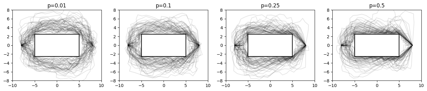
Changing this bias leads to very different trees when expanding towards the goal. The example below shows the solution path (in orange) and the tree that was explored (in blue) for a two dimensional masspoint in empty space for different values of \(p\):
1 Here (pdf) is a paper on the explicit incorporation of that problem in RRTs ('Balancing Exploration and Exploitation in Motion Planning').
Now, in this trivial example we obviously do not need a lot of exploration, since there is no obstacle to avoid. It is however a very good demonstration of the exploration/explotation dilemma.1
Having this tuning parameter lead to the obvious question: How big should the goal bias be? Is there an optimal value for it that is usable over a wide range of problem settings? Obviously, we do not only want to expand the trees towards the goal, as the direct way can be obstructed. However, if too little goal bias is used, we explore the domain unnecessarily long before finally reaching the goal.
How do the resulting paths with different goal biases look like for a simple rectangular obstacle in the middle of the environment?
2 For the optimizer, only the homotopy that we are in matters, the exact path is not that important here. We assume that the optimizer will converge to the same path in any case.
In addition, we take a brief look at the resulting path length, and the computation times of the solutions. Path length is a secondary (but interesting) factor here, since we are usually more interested in the homotopy of the path, and less the exact length, since the path is usually post processed (e.g. smoothed, a velocity profile is added) anyways2.
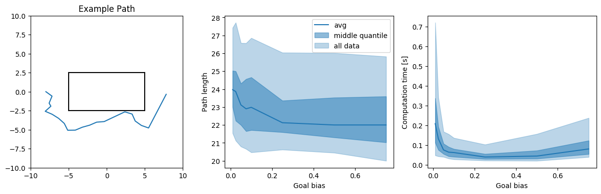
We see that, while the path tends to be ‘more optimal’ (=shorter, in this case), the worst case (and also the average) computation time goes up again if the goal bias is chosen too big. Conversely, if the goal bias is too small, the exploration phase goes on too long, and the paths tend to be a bit longer as well.
3 All experiments were run 100 times for each goal bias. Everything was implemented in python, meaning that it is generally slow (but all experiments are equally slow, so they are compareable).
Ideally, we would look at all possible environments, and planning problems, and run tests on them. Since that is not possible, we try to look at a few different ones3 (hopefully covering some interesting cases):
- A masspoint in an 2D environment with random obstacles
- A masspoint in an 2D environment with a narrow passage off center
- A rigid (L-formed) body in an 2D environment with a narrow passage off center (leading to a 3D problem, with a narrow passage)
- A robotic arm with 3 joints on an axis (i.e. a 4D problem)
- A 6 dimensional masspoint with a (6d)cube in the middle of the environment
We look at the average and the middle quantile (i.e. 25%-75%) of the data of the resulting path length and computation times. Additionally, we plot ‘all data’, i.e. the 5%-95% interval, meaning we get rid of extreme outliers here.
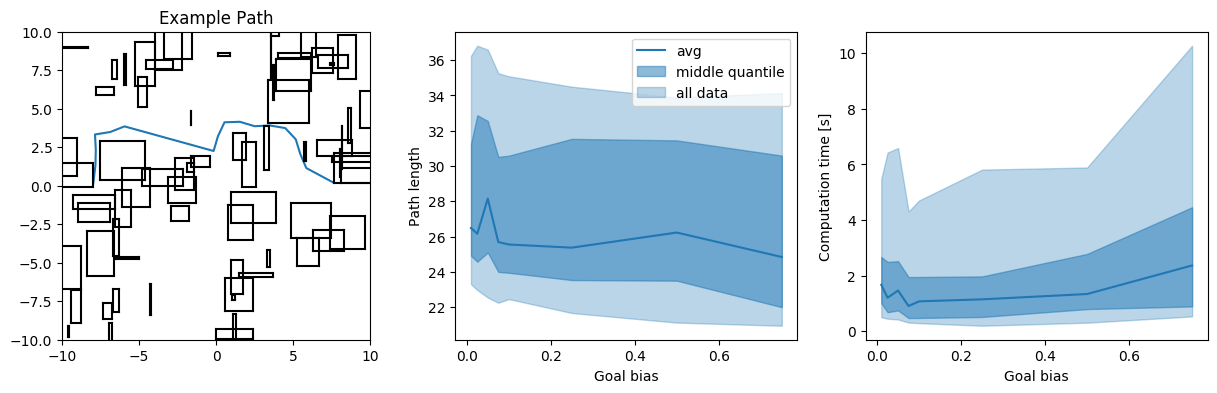
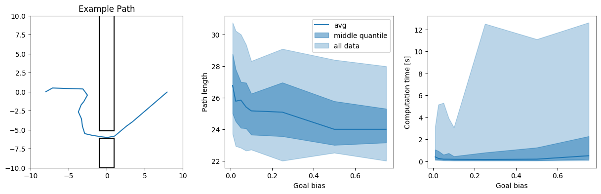
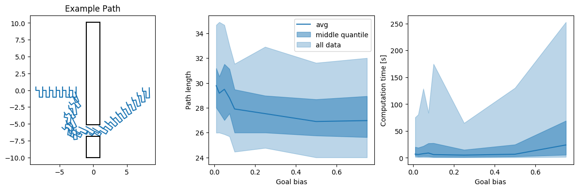

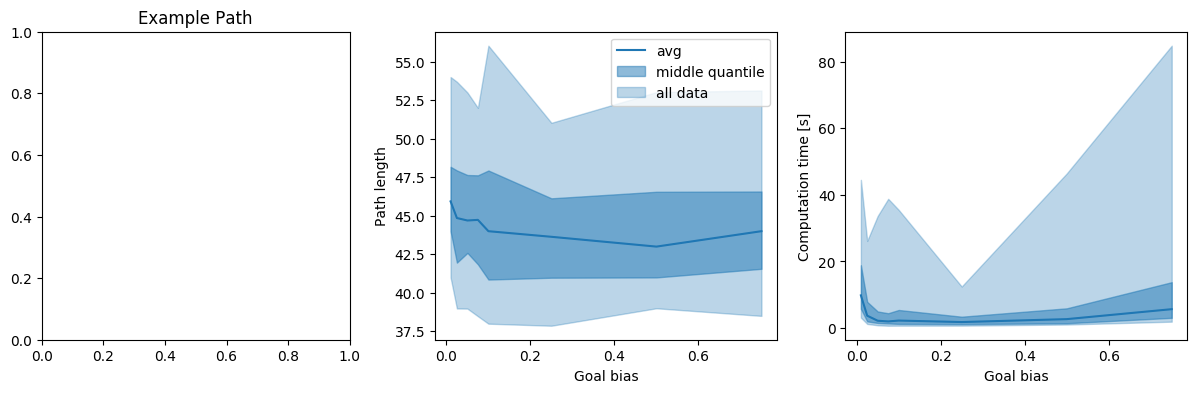
Generally, we are mostly interested in the worst case scenario, not really in the average. It is left to say that this represents the worst case scenarios that occurred during my runs - since it is a probabilistic algorithm, it is always possible to get something even worse with an awful runtime. However, the relations between the different goal biases give a good indicator of how the algorithms tend to perform.
In all of the examples, it is obvious that the extreme values for \(p\) are not exactly a great idea. Additionally, the narrow corridor example shows that there is a benefit in having a tendency for more exploration in case tight passages are present in the path planning problem.
Conclusion/Disclaimer/Discussion
There are a couple of things to keep in mind here:
- None of the examples are really high dimensional problems. Working with e.g. multiple agents, or doing kinodynamic planning leads to higher dimensionalities quickly, and possibly different problems/conclusions
- Other versions of RRT exist - as such a basic RRT implementation can almost always be outperformed by e.g. a bidirectional version of RRT, or a more informed planner.
- More sophisticated versions of goal biasing were not tested. It might be best to first use a very low bias to facilitate good initial exploration, and then gradually increase it to go towards the goal more quickly (hopefully).
In general, it seems to be the case that we want to choose a goal bias of around 5-15% to be safely away from extremely bad performance. However, it is usually possible to run the problem a few times before hand with various parameter settings - meaning it is possible to do this analysis briefly before actually deploying/using the algorithm.