Producing high quality paths: Partial shortcutting
Four years into my PhD, it is the perfect time to start questioning if some of the things that I implemented in the beginning are actually good or if things could be done better. Better in this case is mostly related to 'faster'. Specifically, we are going to be looking at my implementation of path-shortcutting.
In path planning, a common approach is using a fast planner (often RRT-Connect) that produces a valid path that has a relatively high cost, and then using this as basis for further refinement. Particularly, RRT-Connect (or most other sampling based solutions) produce very jagged paths, since the points that make out the path are randomly sampledFor a brief intro to how RRT-Connect works, see the original paper, it is very approachable in my opinion. .
There are a variety of methodsA solid collection is implemented in OMPL. to improve such a path after the initial planning - in this post, we are looking at shortcutting, respectively partial shortcutting.
Code for the following experiments and implementations of methods is available here.
Shortcutting
From here on, we assume that the path is given by a sequence of nodes which are connected by straightline pathsThis is a great assumption if we are looking at robots that operate without kinodynamic constraints and we are doing geometric path planning. It is less great if we are looking at the dynamics of a robot as well. . A simple (but extremely effective) approach to post-process such a path is to shortcut it, that is, taking two (random) points on the path, and trying to connect them with a straight line, as illustrated below.
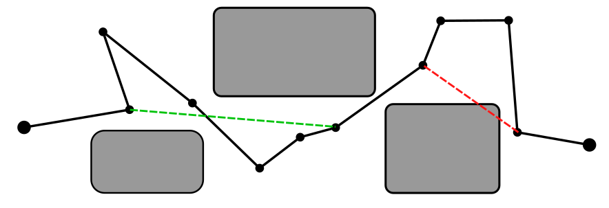
Here, the green shortcut is a valid one (since the new part of the path does not intersect with the obstacles), and the red shortcut is invalid (since it intersects one of the obstacles). This procedure can be done either for a fixed number of iterations, or until some metric is satisfied. In the example above, I chose both shortcuts to start and end in a corner. Typically, this is not the case when implementing a shortcutter: One usually discretizes the path more finely, and chooses two random indices to connect. In pseudocode, shortcutting looks like this:
1
2
3
4
5
6
7
8
9
10
11
12
13
14
15
16
17
18
19
20
def interpolate(path):
    q0 = path[0]
    q1 = path[-1]
    edge = []
    for i in range(len(path)):
        edge[i] = q0 + (q1-q0) * i / len(path)
    return edge

def shortcut(path, collision_resolution, discretization_resolution, max_iterations):
    discretized_path = discretize_path(path, discretization_resolution)
    for _ in range(max_iterations):
        # choose two random points
        i = rnd() % discretized_path.N
        j = rnd() % discretized_path.N

        edge = interpolate(discretized_path[i:j])
        if length(edge) < length(discretized_path[i:j]) and valid(edge, collision_resolution):
            discretized_path[i:j] = edge

    return discretized_path
In many cases, this removes the redundant back and forth that is typical for a plan from a sampling based motion planner very effectively. There are various variants of the proposed algorithm above, such as
- Path pruning, which only considers the discrete points (i.e. the dots in the example above), and not the intermediate configurations to choose places to cut (more formally described here).
- Instead of simply doing a strightline connection, one could run a local planner between two points as described here.
- Instead of uniformly discretizing the path, the work here suggests a way of adaptively discretizing the path.
- Instead of randomly choosing points on the path (as e.g. described here), one can choose them deterministically (see here)
Partial Shortcutting
An issue with normal shortcutting is that all dimensions are shortcut simultaneously. This can lead to some redundant motions that can not be shortcutted. A nice example for this is in the figure below (from the original paper linked above), where a robot with an orientation and a 2d position is used. The rotational-component of the path can not be changed in this example, since the positional component can not be shortcutted.
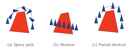
A solution to this problem is shortcutting each dimension separately as seen above on the rightmost illustration, where only the rotational-dimension is shortcut, but the other two dimensions follow the same path from the original solution.
1
2
3
4
5
6
7
8
9
10
11
12
13
14
15
16
17
18
19
20
def interpolate_single_dimension(path, index):
    edge = []
    for i in range(len(path)):
        edge[i] = path[i]
        edge[i][index] = path[0][index] + (path[-1][index]-path[0][index]) * i / len(path)
    return edge

def shortcut(path, collision_resolution, discretization_resolution, max_iterations):
    discretized_path = discretize_path(path, discretization_resolution)
    for _ in range(max_iterations):
        # choose two random points
        i = rnd() % discretized_path.N
        j = rnd() % discretized_path.N
        dim = rnd() % path[0].N

        edge = interpolate_single_dimension(discretized_path, dim)
        if length(edge) < length(discretized_path[i:j]) and valid(edge, collision_resolution):
            discretized_path[i:j] = edge

    return discretized_path
However, while this usually leads to a shorter final path, this approach might take many more iterations for the same shortcut in case a shortcut is actually feasible for all dimensions at the same time. For this reasonAnd possibly some misunderstanding/misremembering of the actually proposed method , at the beginning of my PhD, I implemented a method that randomly samples a set of indices from the dimensions to shortcut, and then shortcuts those indices:
1
2
3
4
5
6
7
8
9
10
11
12
13
14
15
16
17
18
19
20
21
22
23
24
25
def interpolate_subset(path, indices):
    edge = []
    for i in range(len(path)):
        edge[i] = path[i]
        for j in indices:
            edge[i][j] = path[0][j] + (path[-1][j]-path[0][j]) * i / len(path)
    return edge

def shortcut(path, collision_resolution, discretization_resolution, max_iterations):
    discretized_path = discretize_path(path, discretization_resolution)
    all_indices = [i for i in range(path[0].N)]
    for _ in range(max_iterations):
        # choose two random points
        i = rnd() % discretized_path.N
        j = rnd() % discretized_path.N

        num_indices = rnd() % path[0].N
        random.shuffle(all_indices)
        indices = all_indices[:num_indices]

        edge = interpolate_subset(discretized_path, indices)
        if length(edge) < length(discretized_path[i:j]) and valid(edge, collision_resolution):
            discretized_path[i:j] = edge

    return discretized_path
I recently stumbled upon the original paper again, and wanted to double check how my implementation performs against the one that is originally proposed in the paper. I am mostly interested in convergence of the method, respectively computation speed.
Experiments
The methods that we will compare are a selection of the things above:
- pruning
- shortcutting
- partial shortcutting (with a single dimension at a time)
- partial shortcutting (with a random subset of dimensions)
I run all the methods on a few different scenarios, and report the results below. For each of the scenarios, I used RRT-Connect to produce an initial path, and then run the methods above to postprocess the path.
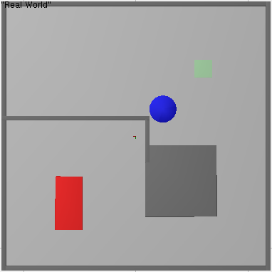
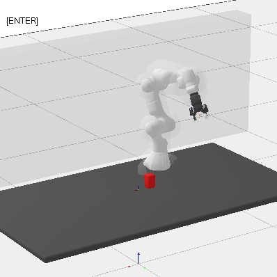
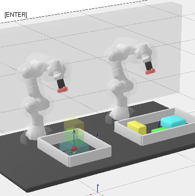
Since I am mostly interested in manipulation planning, the scenarios I am using are from previous papers of mine, and will contain things to be manipulated. Particularly, I am going to be looking at multiple paths in the same environment, where the agent is moving things around (e.g. a path that leads to a robot picking something up and a path that leads to some placement position).
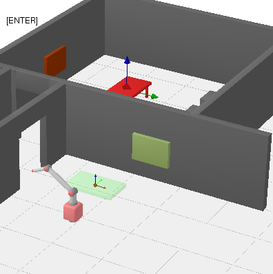
Conretely, the scenarios are i) a simple 2d scenario with obstacles where a ‘sofa’ has to be moved through a narrow corridor, ii) a robotic manipulator on a table with an object that has to be rotated, iii) two robot arms that perform a handover, and iv) a mobile manipulator that has to move an actual table to a different roomObviously, this is not a perfect test of the methods, but my intuition tells me that this should paint a sufficient picture. There are more experiments in the github repo where the code lives. :
Below, I plot the path length against the compute time. I ran all the shortcutters 50 times. The thick line is the median of all runs for that specific method and the shaded area in the same color is the 95% non-parametric confidence interval. The x axis is computation time, and the y axis is path length in all of the plotsOpen the plots directly in a new window/tab to see them in mauch larger. .
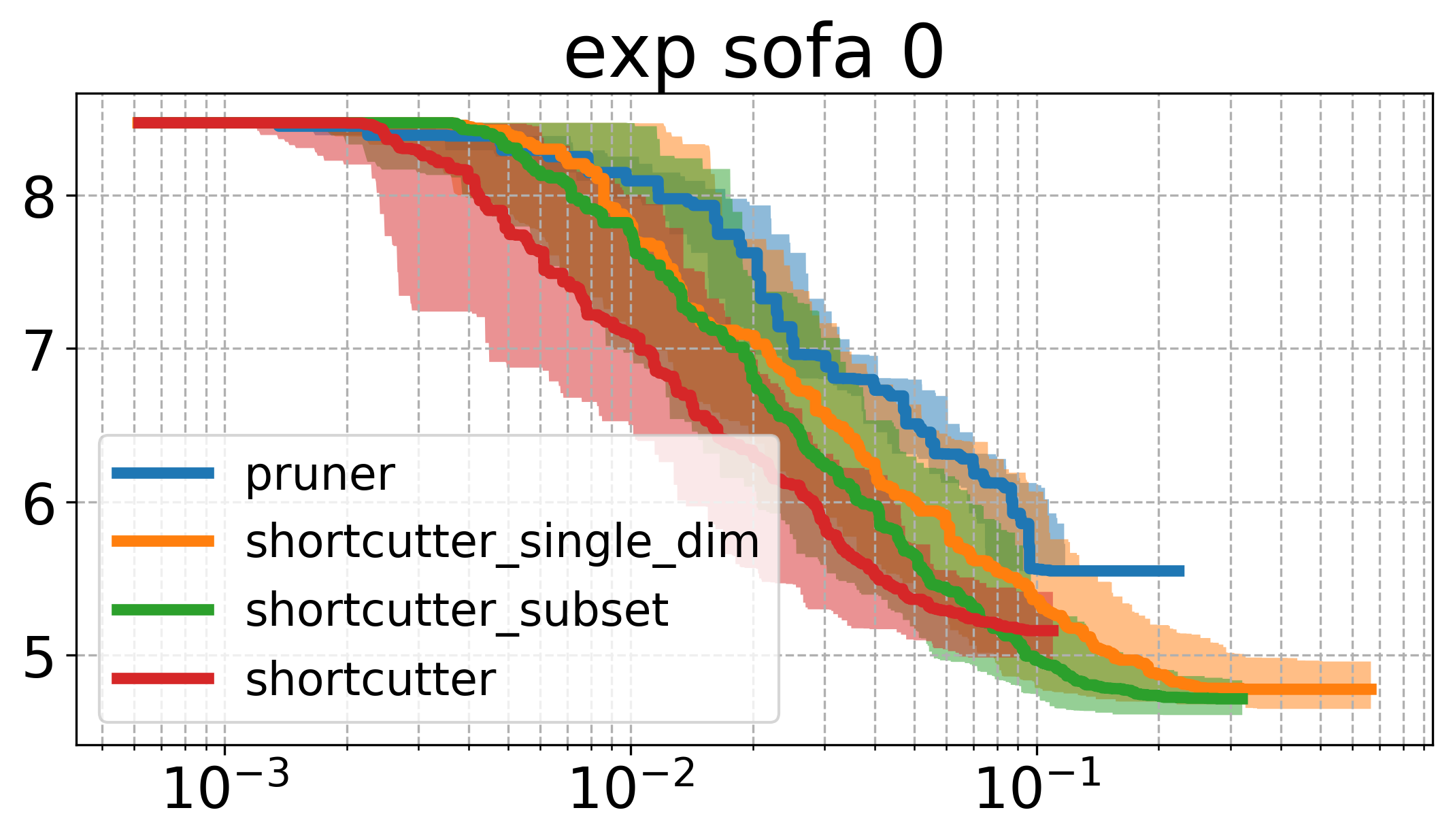
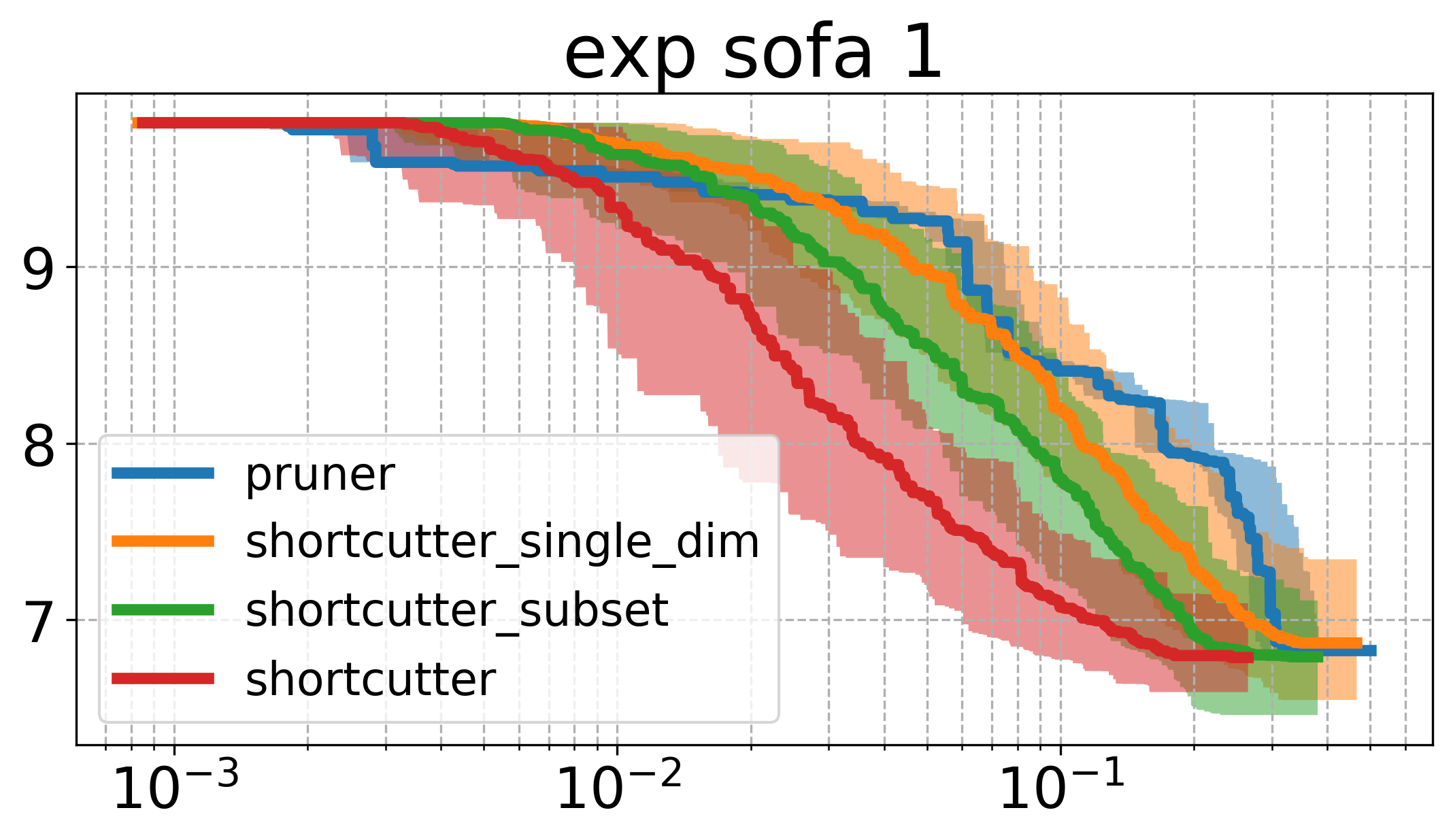
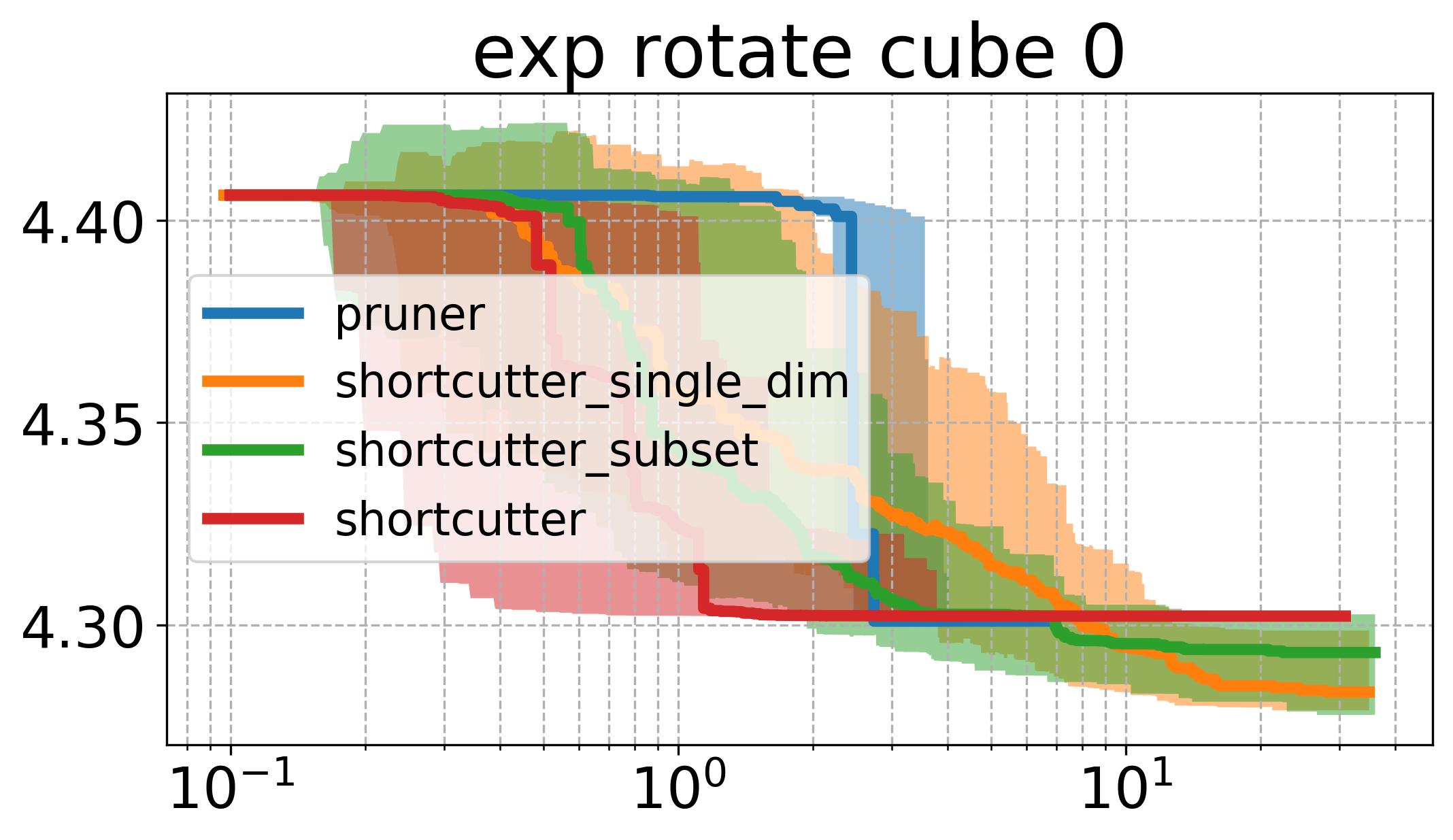
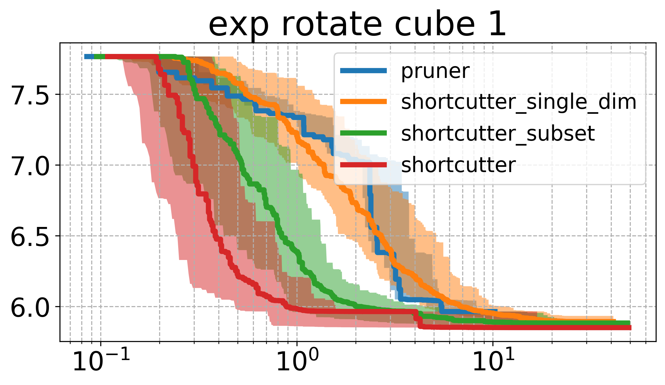
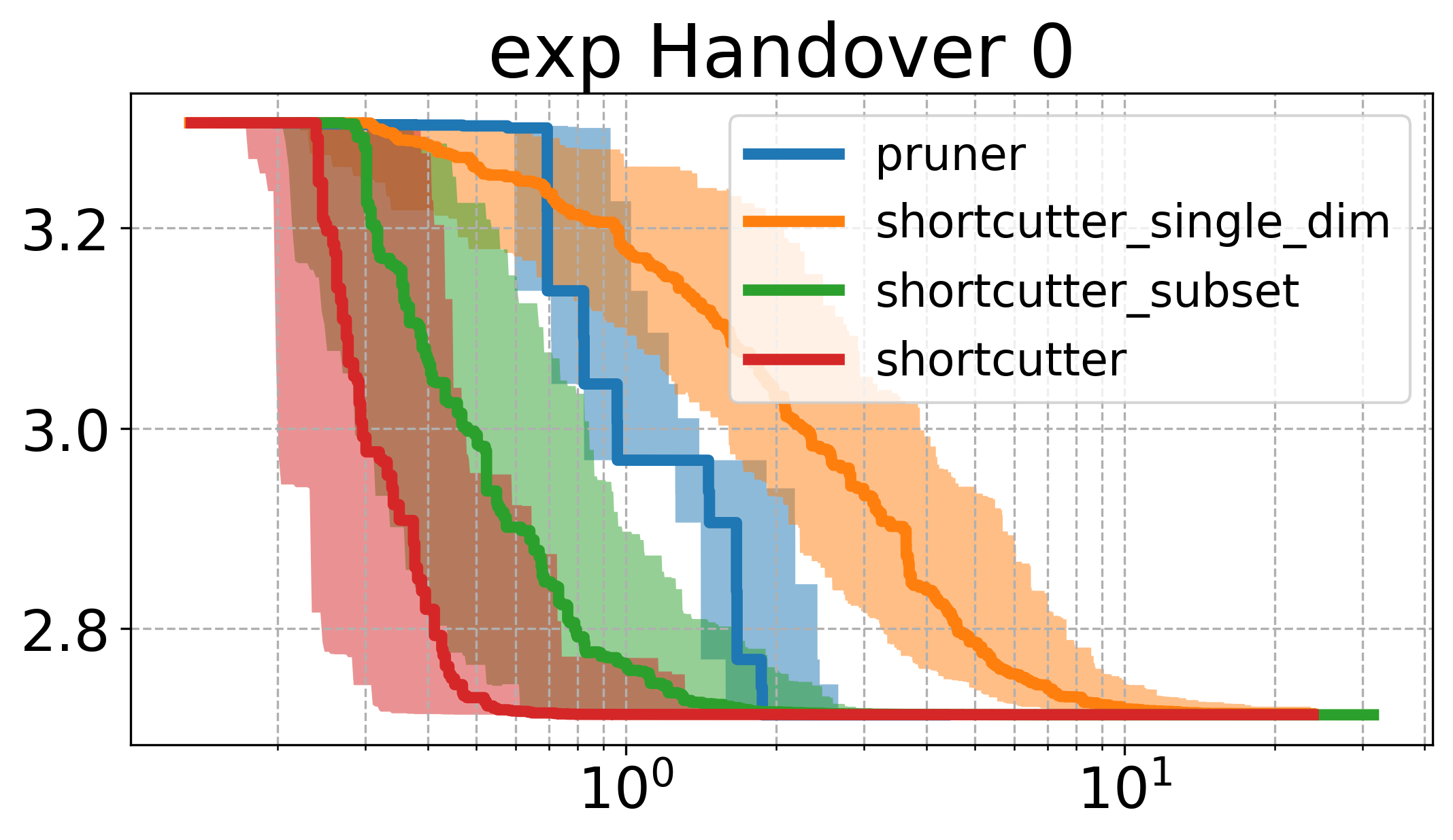
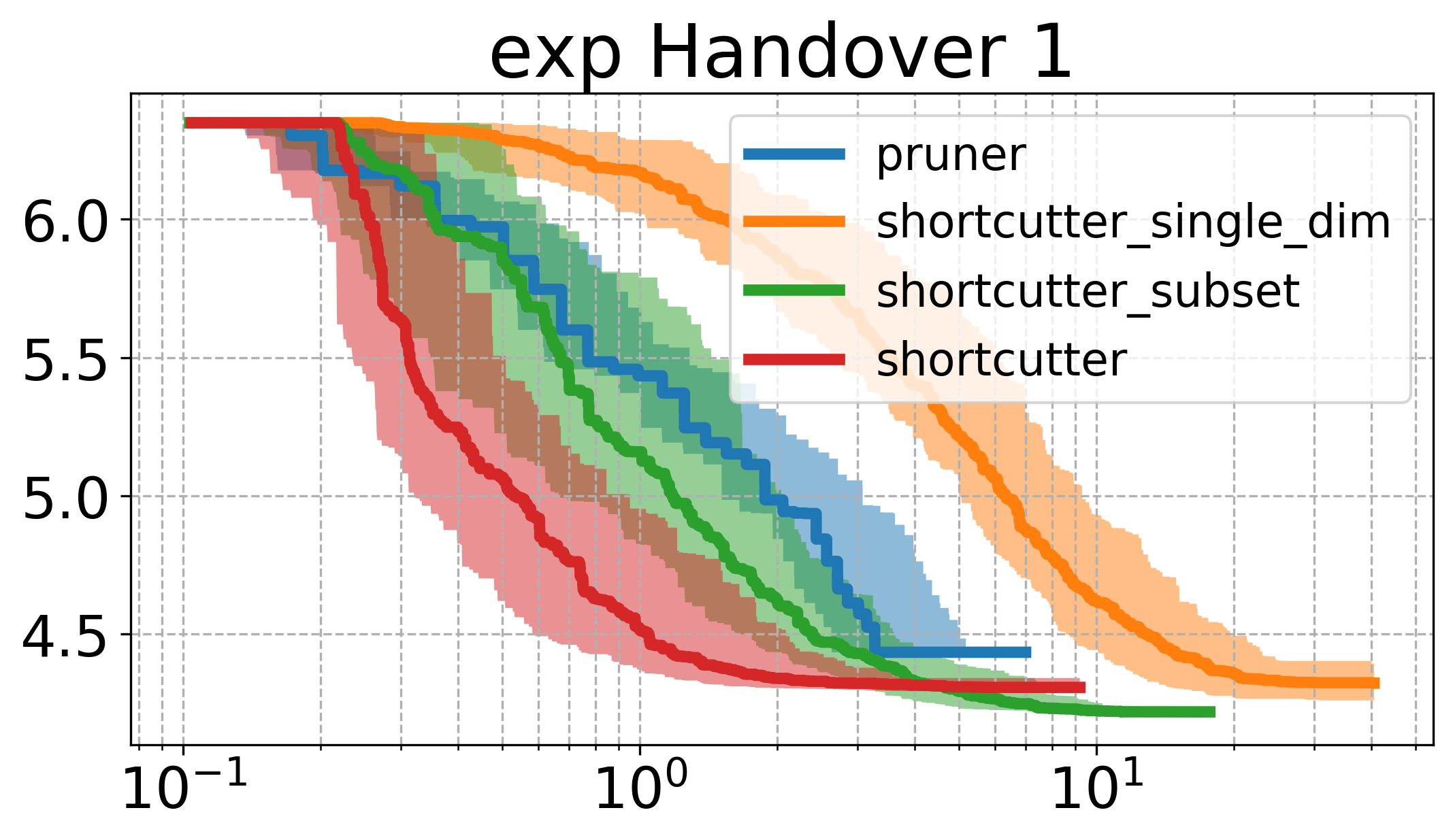
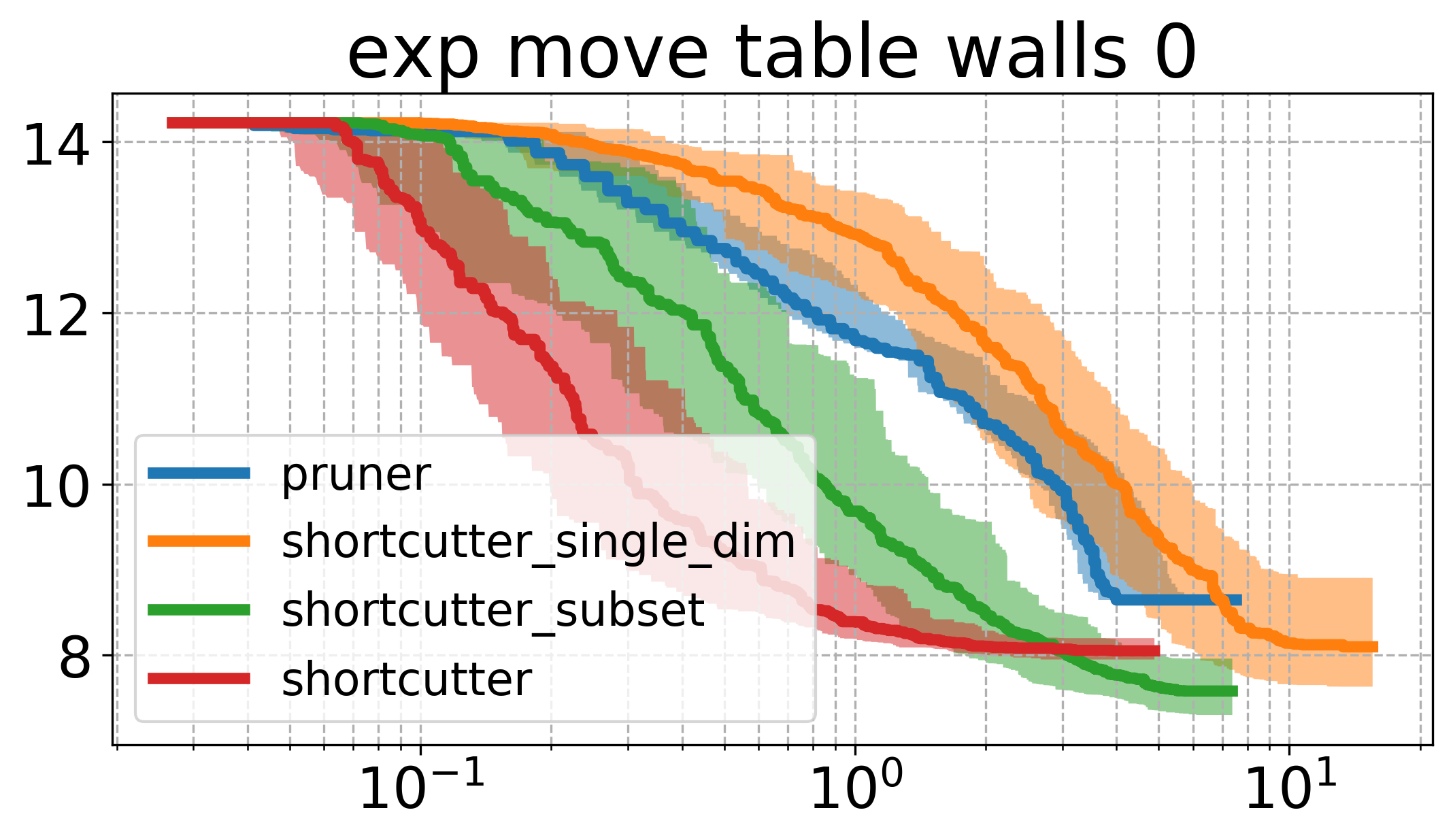
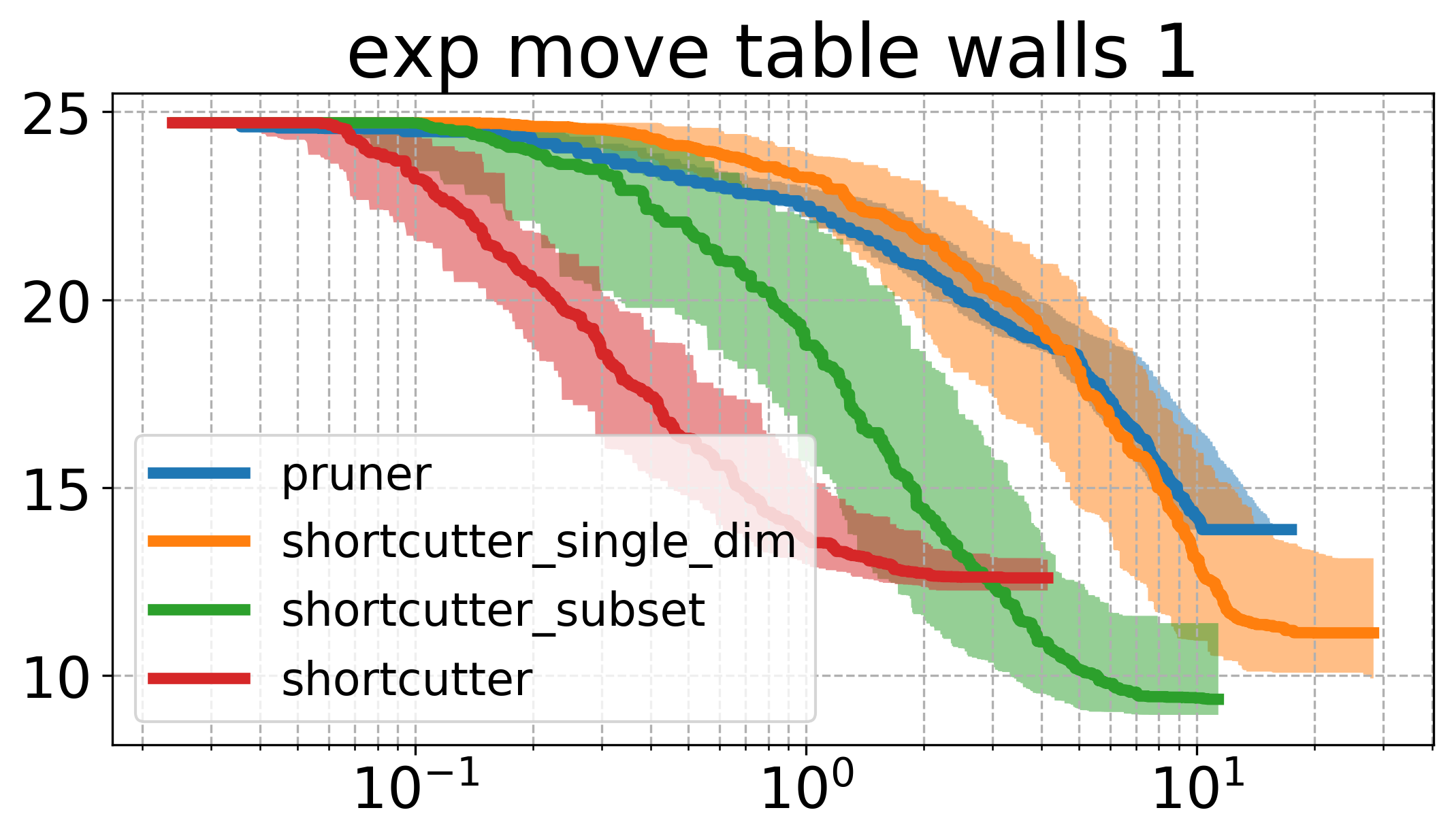
The first thing to notice is that the plots above are very different from the ones shown in the original paper. Partial shortcutting with only a single dimension seems to be slower than normal shortcutting in quite a few of the cases. This might have to do with the type of problem we are looking at though. When focussing on the experiments (a) and (f) of the original paper (a planar corridor, and a manipulator), a similar effect can be seen as the one we have here (i.e. the shortcutter is faster than the single-dimension shortcutter in the original experiments as well). It does however, typically get similar or the lowest cost of the tested methods.
In the plots above, the subset-shortcutter is only slower than the normal shortcutter, but finds paths with similar or shorter lengths as the single-diemension shortcutter. Further, the expected effect appears for the shortcutting and the pruning, namely that they do not get the path length as low as the other two approaches.
Ablations
In additon to the experiments above, I wanted to add a few ablations that show which things matter, respectively things that I learned during these experiments.
The first one is how we discretize a path: Since we want to look not only at the corners of the path for shortcutting, we typically discretize the edges between them more finely, such that we can simply sample random indiceds for shortcutting afterwards.
However, too finely discretizing the path will sometimes lead to extremely small improvements in path cost while incurring the cost of checking the validity of the whole length of the new edge. Conversely, not discretizing the path finely enough will lead to a limitation in how much the path can be improved. Thus, there must be some kind of optimum for the discretization resolution.
The following two plots are with different discretizations of the path.
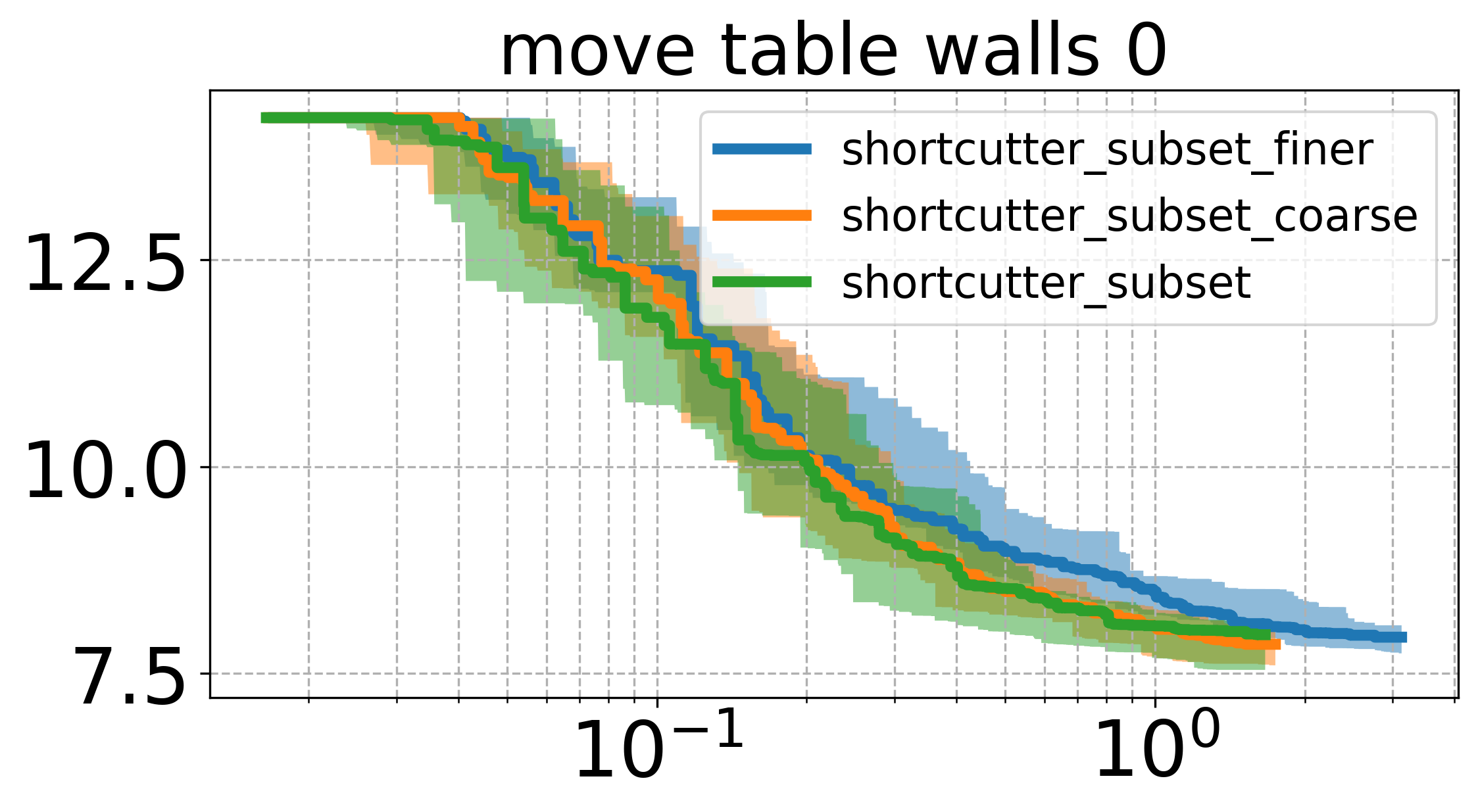
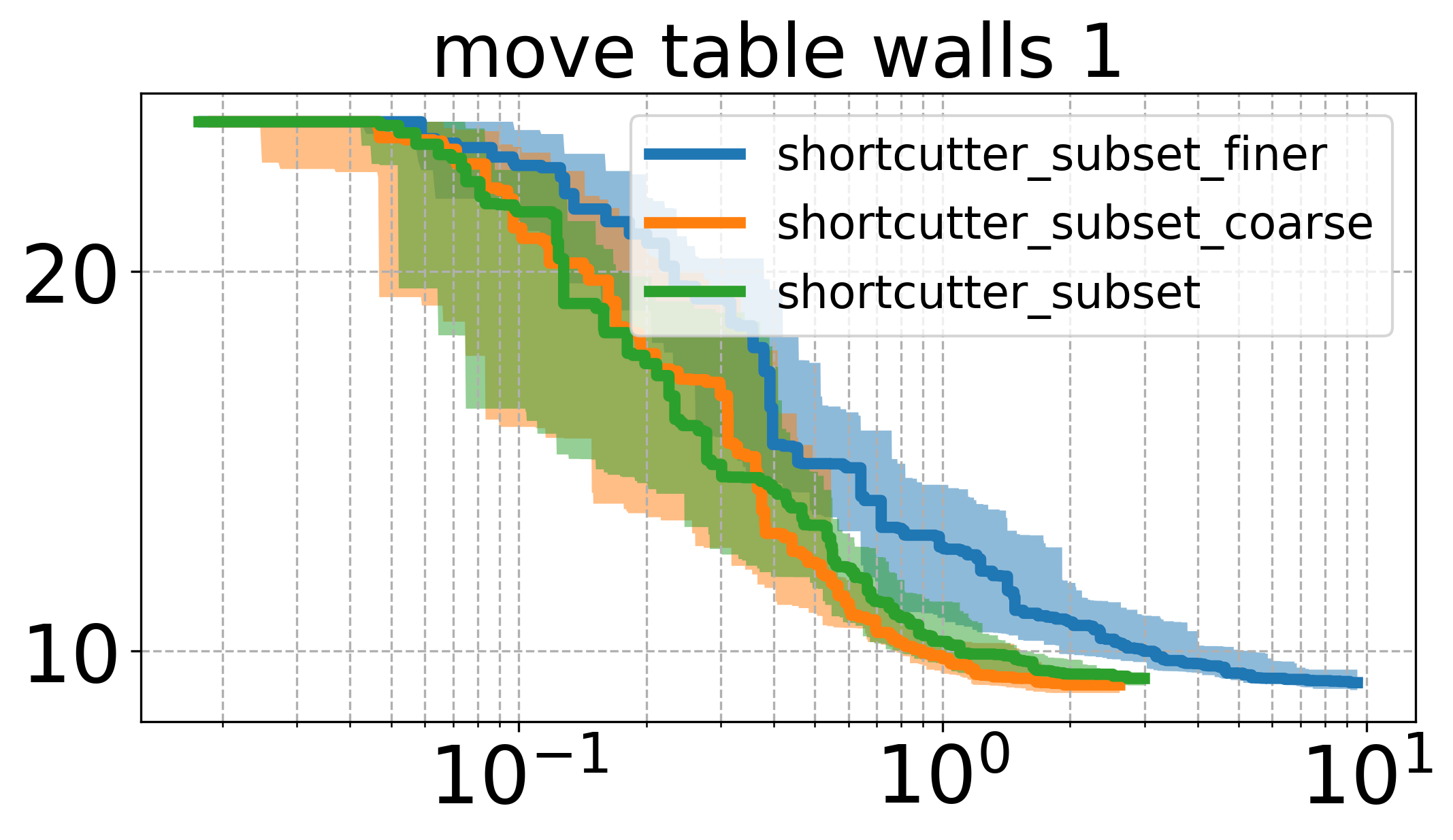
These plots show that while there is a bit of a difference between different discretizations, they are not too drastic.
Additionally, there is a conflict with collision checking when discretizing the path. Collision checking of a path typically works by discretizing the path into some defined resolution, and then collision checking these states. Now, if the path is too finely discretized (finer than the collision checking resolution), this leads to many more collision checks that are done on the path compared to only checking at a certain resolution.
This problem is easy to avoid if one implements the interpolation function carefully, and one is aware that this issue can arise.
The second thing I want to look at briefly is how to sample indices to shortcut: In the implementation above, I tried to get a uniform sampling scheme, by first uniformly sampling the number of indices, and then randomly choosing the indices.
A different approach for sampling indices could be iterating through the indices, and adding an index to the subset with a certain probability. Comparing the uniform sampling and the approach described above gives the plots below:
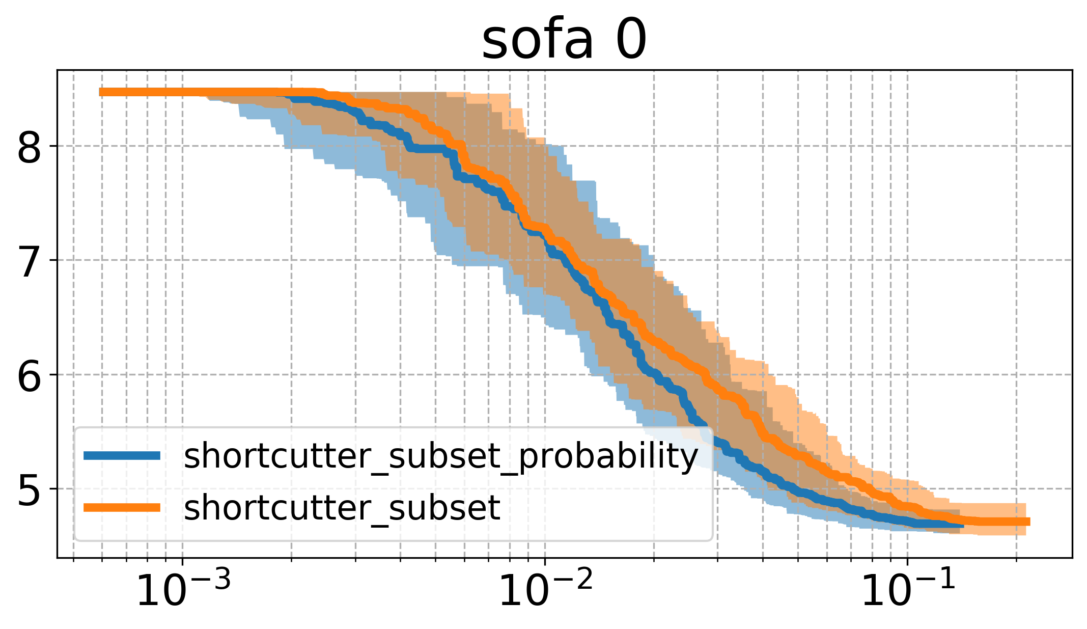
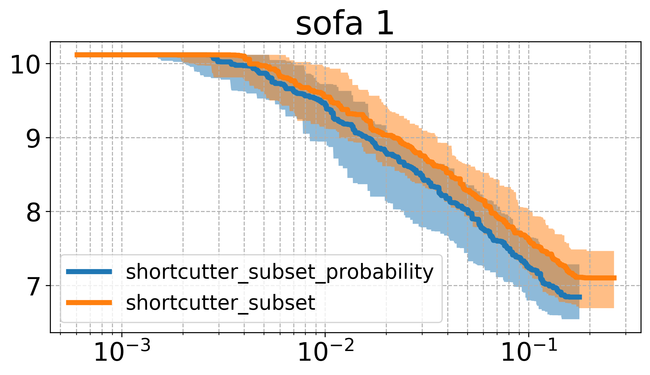
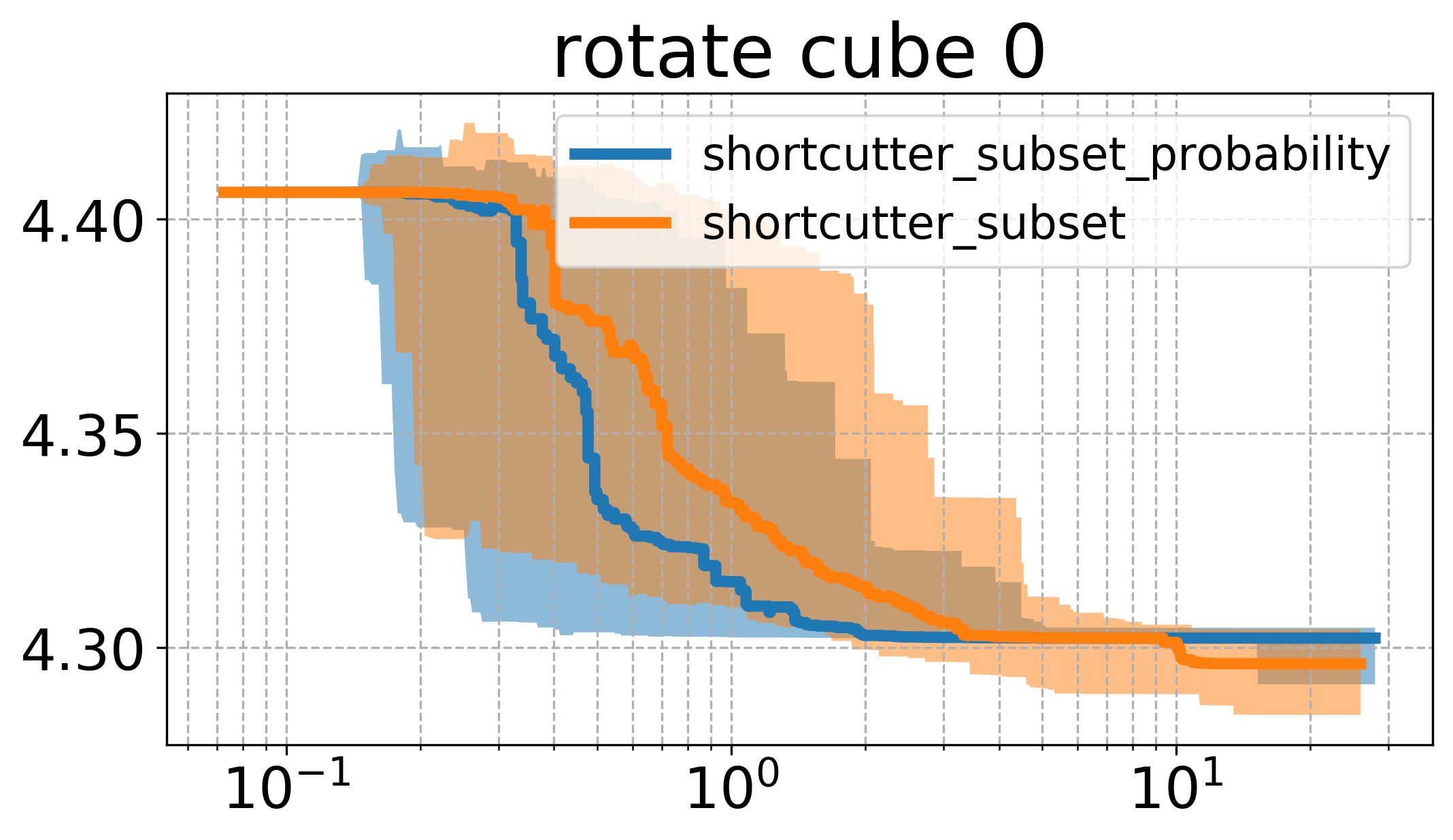
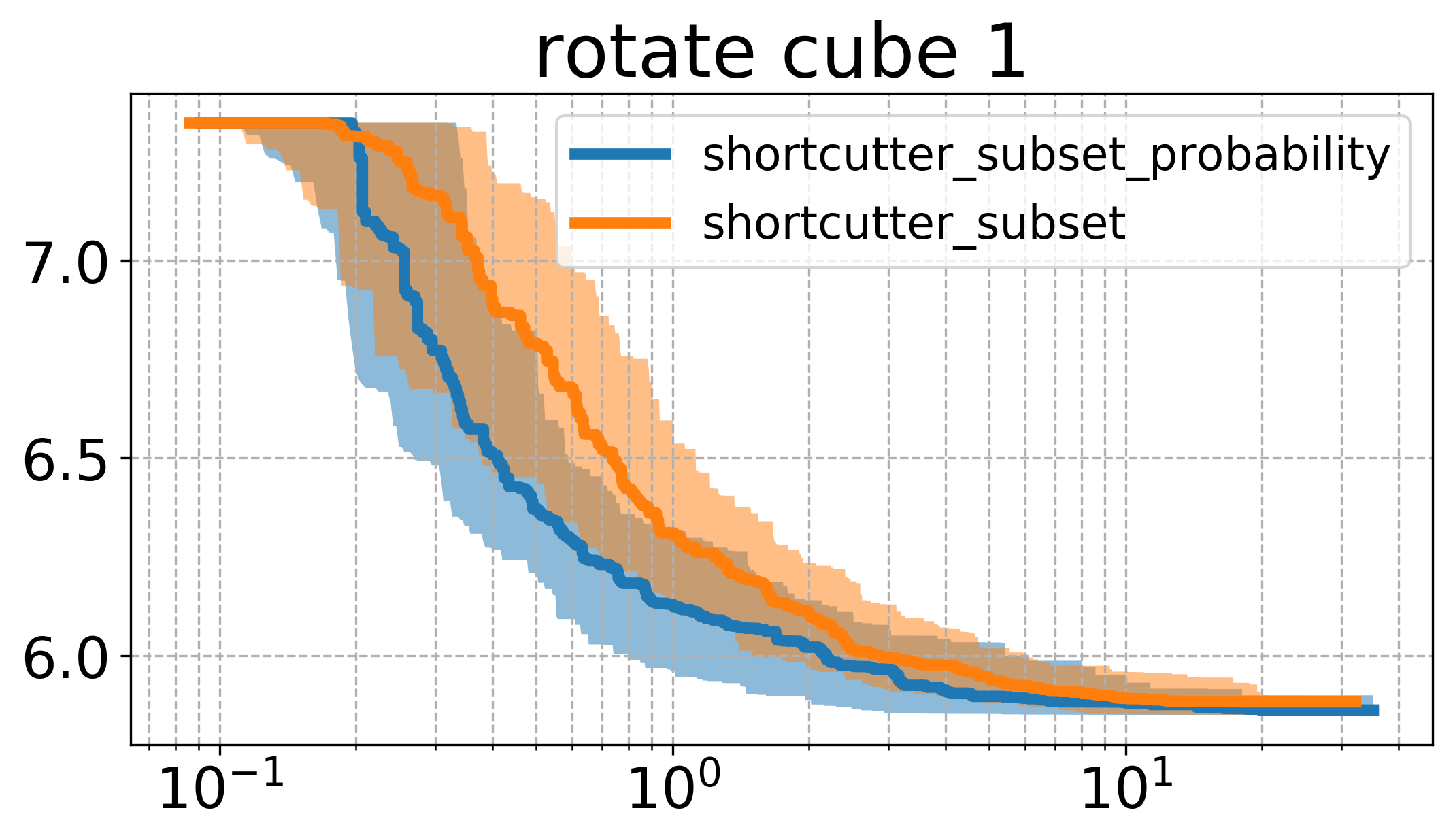
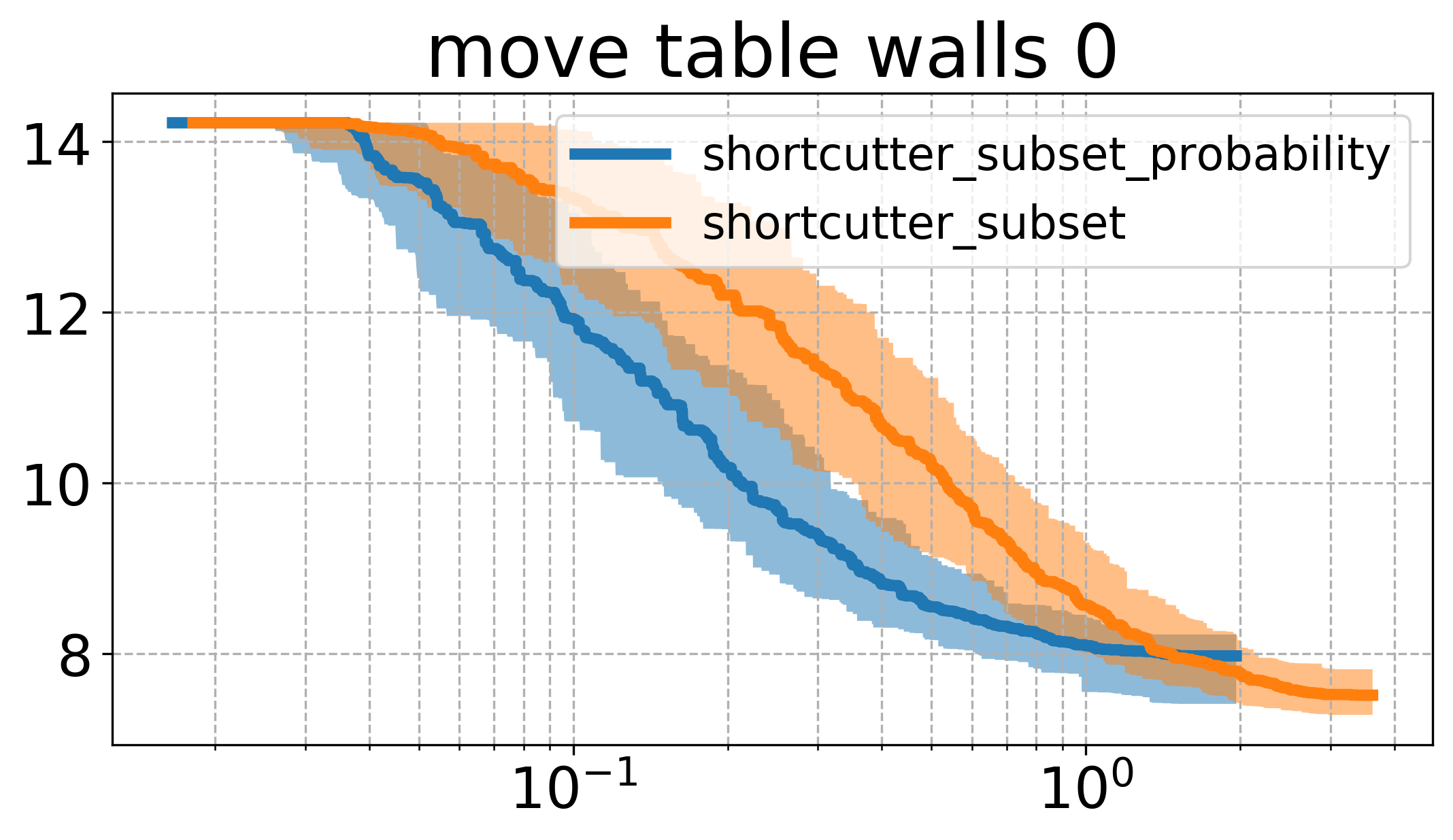
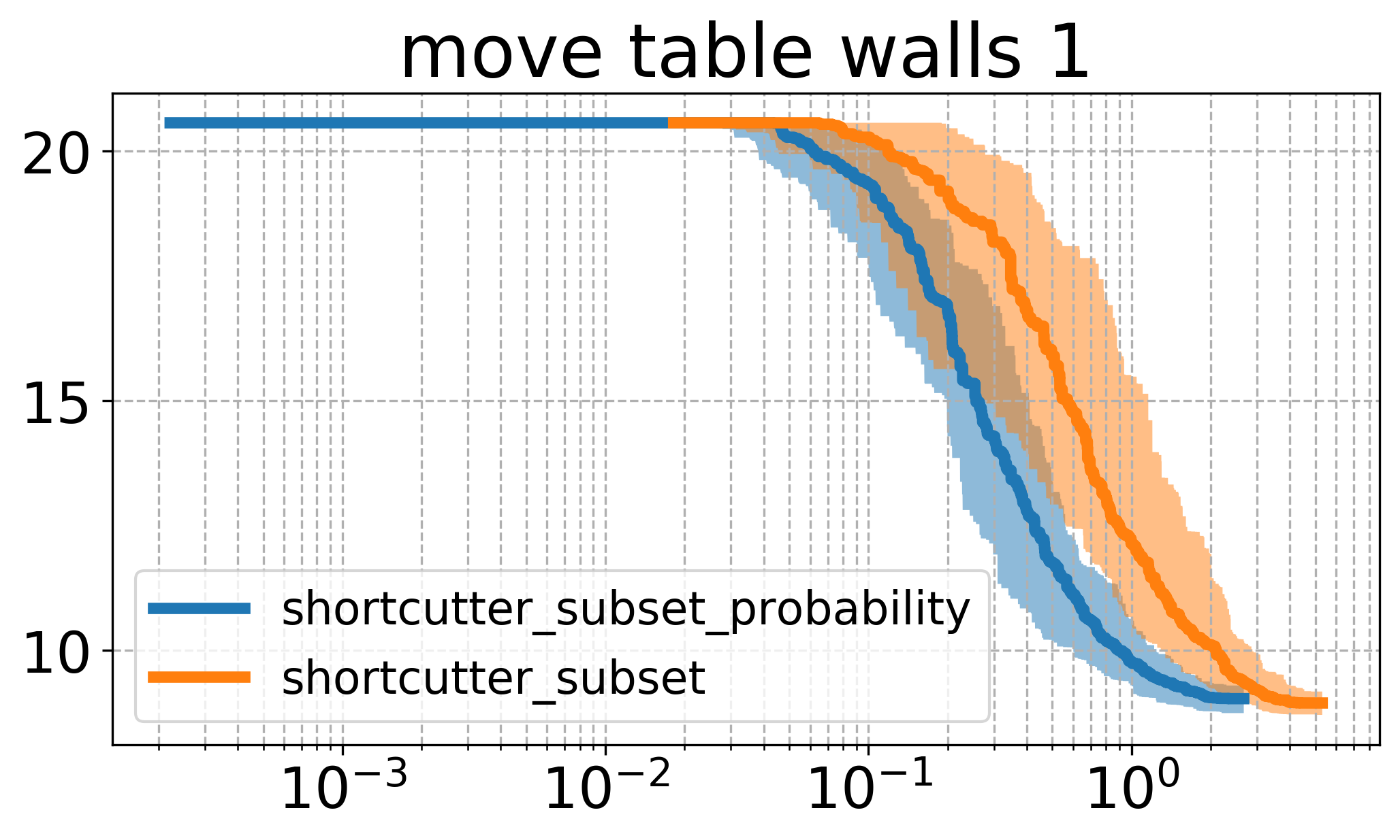
Here, it can be seen that there seems to be a quite big influence of how we sample, namely that the higher probability to sample a larger set of indices leads to faster runtime in this case. Comparing the plots here with the one above, one can see that this version of sampling indices performs essentially the same as the vanilla shortcutting version, while reaching roughly the same cost as the uniform subset shortcutting.
The result leads me to believe that there might be some better strategy, that is possibly taking into account the history of the process (e.g. trying to shortcut larger sets initially, and later during the process favorably sampling smaller sets).
Takeways
Clearly, there are a few things that one should keep in mind when implementing shortcutting. The thing that surprised me the most (but should be obvious) is that a too fine discretization can lead to unintended problems (your shortcutter being very slow).
Subset-shortcutting seems to be quite a bit better than the single-dimension shortcutting on the scenarios that I care about most, and the performance seems to be similar to the one from the shortuctter that always interpolates all indices.
From the experiments here, I argue that the subset shortcutter is the correct choice if the main concern is speed. That being said, the normal shortcutter seems like very solid choice as well, and is slightly simpler to implement.
Outlook
Clearly, there are a number of design choices in all the implementations above - the choices range from what to sample, what distributions to sample from, which order to sample things in and so on. It is questionable if those design choices represent some sort of optimum. A thing to do then might be to try to find optimal distributions that we sample things from.
Additionally, there are some thigs that can clearly be optimized. If we do shortcutting for only a single dimension, that only changes some of the parts of the robot we are looking at. Thus, we might be able to save some time by only collision checking the parts of the robot that actually changed.
Next, there are a number of things that could be cached here, to avoid e.g., attempting to (unsuccessfully!) shortcut the same thing twice.
Finally, it would be interesting to collect some metrics on where time is spent. From experience, the most time is usually taken by the valid edges (since the validation-attempt of invalid edges typically terminates earlier). From this follows that it would be desirable to avoid the ‘incremental’ improvements, and ideally try to find the big improvements first.