Faster sampling of sum-of-infinity-norm bounded sets
In path planning, the cost function is commonly the path length. This leads to the euclidean norm as distance function. However, if we care about, e.g., planning with a robot arm, and we want to minimize the time that a path takes, the euclidean norm does nor make sense, and we should use the infinity norm. Using the infinity norm for the cost makes some things more annoying. Here is how to solve them.
Sampling based path planning works by uniformly sampling points from a set, and building a tree by connecting the samples. Eventually, a path from the start to the goal is part of the tree. If we do path planning and use the infinity norm as cost, we can not do some fancy things that can be done when using the euclidean norm as cost. One such example is informed sampling.
Code for the plots and timings in this post can be found here.
Informed sampling
In sampling based path plannning, informed sampling is the process of only sampling points that can actually decrease the total cost of the path, which speeds up convergence of the planning algorithms tremendously. That is, given some previously found best path \(p\) and the corresponding best cost \(c_b\), we only want to sample points that can connect thet start and the goal with a cost lower than the already found cost \(c_b\). The set of points that can connect a single start and a single goal with a cost that is lower than \(c\) is Something similar can be written down for multiple starts and goals.
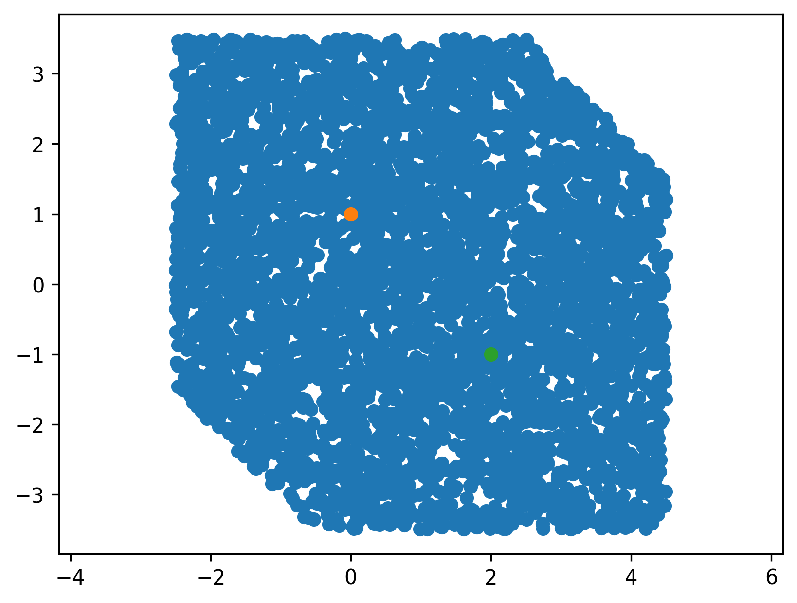
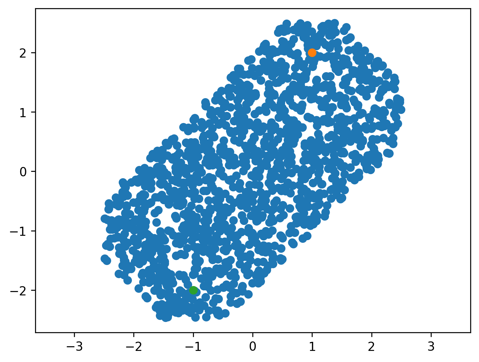
\[\mathcal{X}^* = \{x\in\mathcal{X} |\ f(x, x_s) + f(x, x_g) < c_b\}\]If our cost \(f\) is the euclidean norm, we can do what is described in the paper by Jon Gammell here, which allows for direct uniform sampling of the set. If our cost is the infinity norm, this does unfortunately not workIt also does not work as nicely for multiple starts and goals. . Substituting the infinity norm for \(f\) above, our set becomes
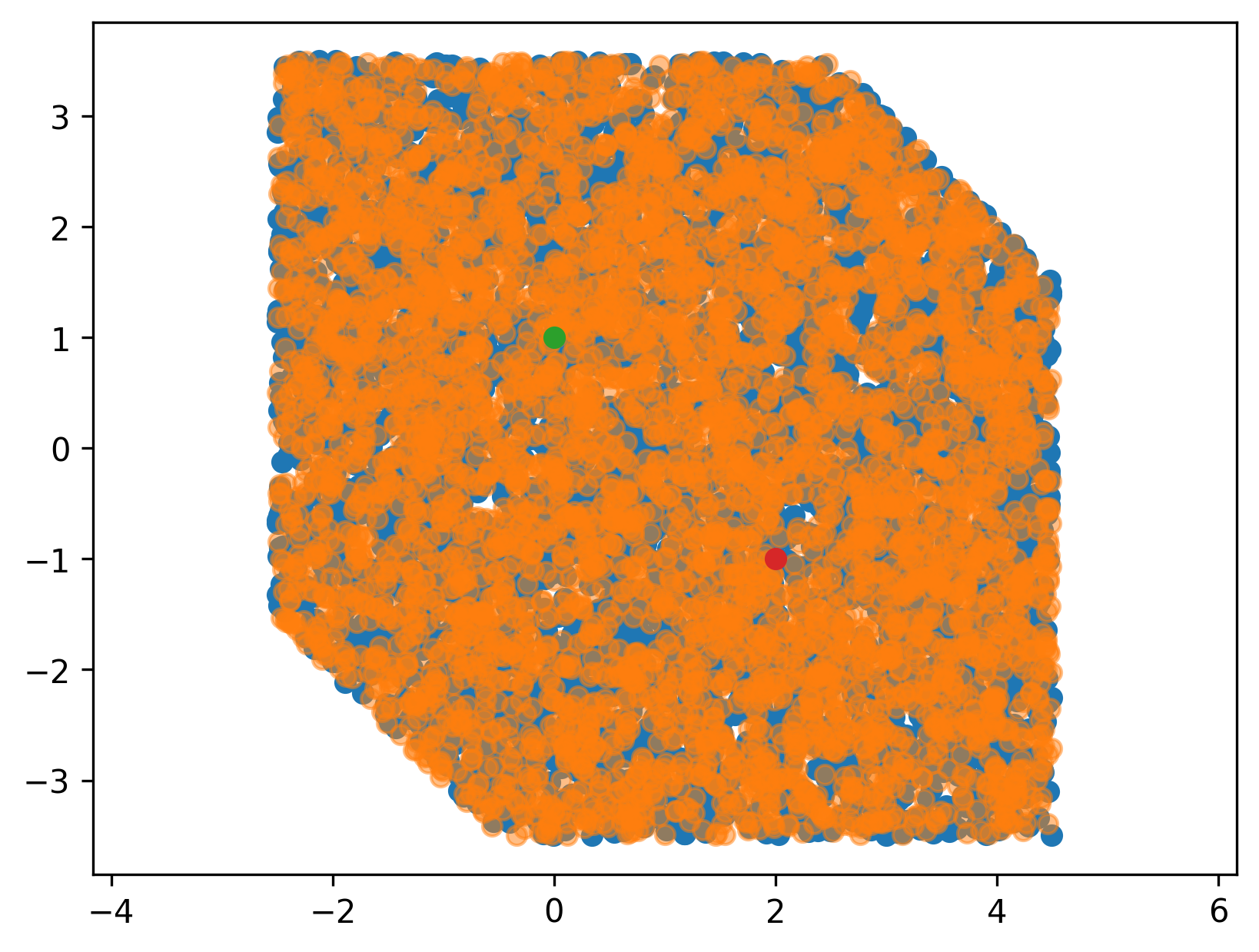
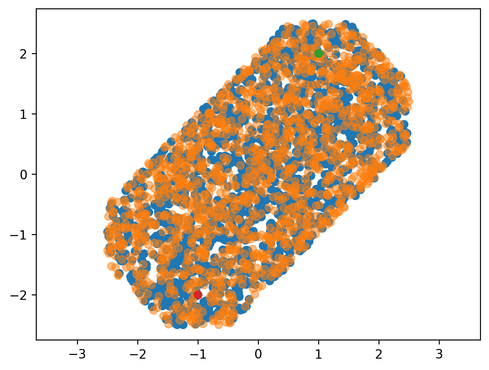
\[\begin{align*} \mathcal{X}^* &= \{x\in\mathcal{X} |\ ||x - x_s||_\infty + ||x - x_g||_\infty < c_b\}\\ &= \{x\in\mathcal{X} |\ \max_i|x_i - x_{s,i}| + \max_j |x_j - x_{g,j}| < c_b\} \end{align*}\]which is a convex polytope (and can be described by the intersection of multiple halfspaces). For two dimensions, it might look like so for different values of \(x_s\), \(x_f\) and \(c_b\)Three dimensions are harder to visualize, but there is an example in the script linked above. :
One possibility to sample uniformly from this set would be rejection sampling, but rejection sampling is typically not even close to direct sampling in efficiency, especially in high dimensions. Dimensionality wise, we are interested in 6 to 14 dimensional problems, as we usually plan for one or two arms with 6 or 7 DoF.
Representing the set as halfspaces
To gain some understanding of the structure of the set we describe the polytope as intersection of halfspaces, i.e., as \(A\mathbf{x}\leq b\). We can convert the set above into this notation by trying to get rid of the absolute value in the constraint above. We can do this by considering different cases, i.e., the case where the index \(i = j\) and \(i \neq j\):
We start with the case where \(i=j\): We begin by introducing the variable transformation \(x' = x - \frac{x_s + x_g}{2}\), i.e., we translate our polytope to be centered around the origin. With this transformation, we get that \(x'_g = - x'_s\). Thus, the constraint for dimension i becomes
\[|x'_i - x'_{s,i}| + |x'_i - x'_{g,i}| < c_b\]respectively \(|x'_i - x'_{s,i}| + |x'_i + x'_{s,i}| < c_b\)
We can then consider two cases to get rid of the absolute value: one where \(x'_i - x'_{s,i} < 0\), and one where \(x'_i + x'_{s,i} < 0\). Taking all this together, we get the constraint
\[-c_b/2 \leq x'_i \leq c_b/2\]i.e. a box constraint. This box constraint represents a box that is centered around the origin, with the sidelength \(c_b\).
In the case where \(i \neq j\), we consider 4 cases to get rid of the absolute value:
\(\vert x'_i - x'_{s,i}\vert < 0,\ \vert x'_j + x'_{s,j} \vert < 0\), which leads to
\[-x'_i + x'_{s,i} - x'_j - x'_{s,j} < c_b \Rightarrow \boxed{-x'_i - x'_j < c_b - x'_{s,i} + x'_{s,j}}\]\(\vert x'_i - x'_{s,i}\vert > 0,\ \vert x'_j + x'_{s,j} \vert < 0\), which leads to
\[x'_i - x'_{s,i} - x'_j - x'_{s,j} < c_b \Rightarrow \boxed{x'_i - x'_j < c_b + x'_{s,i} + x'_{s,j}}\]\(\vert x'_i - x'_{s,i}\vert < 0,\ \vert x'_j + x'_{s,j}\vert > 0\), which leads to
\[-x'_i + x'_{s,i} + x'_j + x'_{s,j} < c_b \Rightarrow \boxed{-x'_i + x'_j < c_b - x'_{s,i} - x'_{s,j}}\]\(\vert x'_i - x'_{s,i}\vert > 0,\ \vert x'_j + x'_{s,j}\vert > 0\), which leads to
\[x'_i - x'_{s,i} + x'_j + x'_{s,j} < c_b \Rightarrow \boxed{x'_i + x'_j < c_b + x'_{s,i} - x'_{s,j}}\]where the left side of the equation gives us the coefficients of the matrix \(A\), and the right side gives us the entries in \(b\). Taking this together, we can construct the matrix \(A\) and the vector \(b\) like so:
1
2
3
4
5
6
7
8
9
10
11
12
13
14
15
16
17
18
19
20
21
22
23
24
25
26
27
28
29
30
31
32
33
34
35
36
def make_halfspaces(xs, xg, cb):
    N = dim*(dim-1) + 2 * dim
    A = np.zeros((N, 2))
    b = np.zeros(N)

    for i in range(dim):
        for j in range(dim):
            if i == j:
                continue

            A[cnt * 4, i] = -1
            A[cnt * 4, j] = -1
            b[cnt * 4]    = cb - xs[i] + xs[j]

            A[cnt * 4 + 1, i] =  1
            A[cnt * 4 + 1, j] = -1
            b[cnt * 4 + 1]    = cb + xs[i] + xs[j]

            A[cnt * 4 + 2, i] = -1
            A[cnt * 4 + 2, j] =  1
            b[cnt * 4 + 2]    = cb - xs[i] - xs[j]

            A[cnt * 4 + 3, i] =  1
            A[cnt * 4 + 3, j] =  1
            b[cnt * 4 + 3]    = cb + xs[i] - xs[j]

            cnt += 1

    for i in range(dim):
        A[cnt*4 + i*2, i] = 1
        b[cnt*4 + i*2] = cb/2

        A[cnt*4 + i*2 + 1, i] = -1
        b[cnt*4 + i*2 + 1] = cb/2

    return A, b
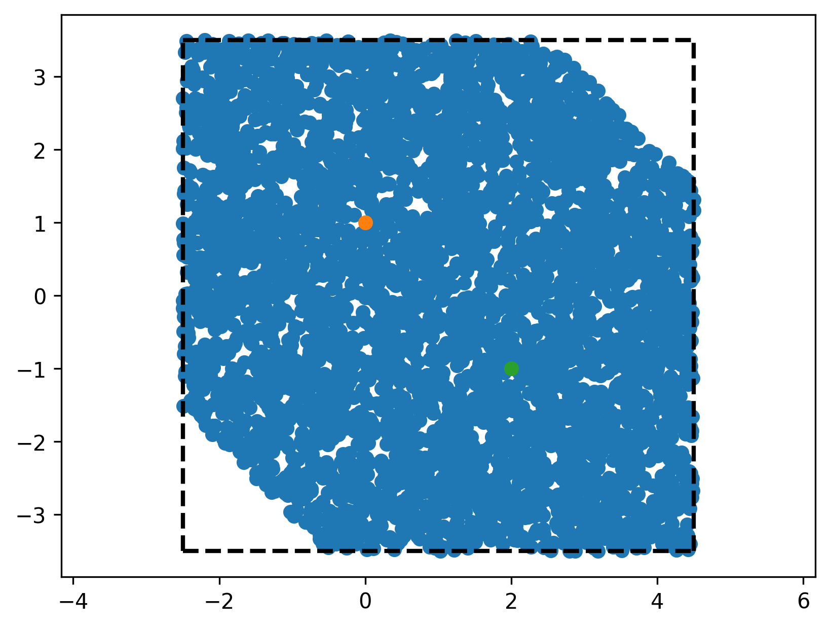
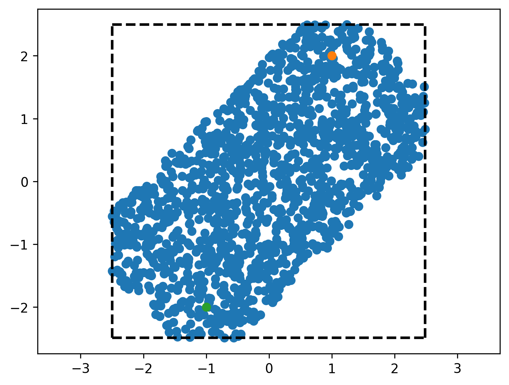
we can use this to confirm visually that we did not mess up any of our transformations (orange dots are the ones where \(Ax < b\), blue dots are directly checked against the condition above).
Finally, it is important to note that we typically have some additional constraints from the robot itself, respectively the states that are actually valid for a robot. These migth come from the joint-limits, or from some other user-imposed constraints. Very often, those constraints are box constraints, and thus can be added quite easily to our \(A\) and \(b\) matrix and vectors respectively.
Sampling from a polytope
Unfortunately, sampling uniformly from a convex polytope is not very straightforward. The obvious (and probably best) approach, is to take the box constraint above, sample from this uniformy, and then do rejection of the points that do not fulfill the constraint.
A different approch would be trying to subdivide the complete polytope into subsets from which we can sample directly, and then first choose a subset to sample from, and then sample from this. Unfortunately, I was not yet able to come up with a good subdivision of the polytope.
Another possibility to produce uniform points from a convex set are random walks. Particularly hit-and-run sampling sounds interesting: This is a random walk based method, and a good explanation can be found here. However, hit and run sampling needs to do many iterations/steps before converging to something that resembles a uniform distribution. Thus, this is unsuitable for our usecase.
Benchmarking
We compare two simple approaches: rejection sampling, and sampling from the box, and then rejection sampling, and consider the computation time to generate N samples.
1
2
3
4
5
6
7
8
9
10
11
12
13
14
15
16
def rejection_sampling(bounds, xs, xf, cb, N=1):
    mean = (bounds[:, 0] + bounds[:, 1]) / 2
    w = bounds[:,1] - bounds[:, 0]

    pts = []
    num_attempts = 0
    while True:
        num_attempts += 1
        x = (np.random.rand(bounds.shape[0]) - 0.5) * w + mean

        d = np.linalg.norm(xs - x, np.inf) + np.linalg.norm(x - xf, np.inf)
        if d <= cb:
            pts.append(x)

            if len(pts) >= N:
                return pts
1
2
3
4
5
6
7
8
9
10
11
12
13
14
15
16
17
18
19
20
21
22
def rejection_sampling_with_box(bounds, xs, xf, cb, N=1):
    cost_min = -cb/2 + (xs + xf) / 2
    cost_max =  cb/2 + (xs + xf) / 2

    mins = np.maximum(bounds[:, 0], cost_min)
    maxs = np.minimum(bounds[:, 1], cost_max)

    mean = (mins + maxs) / 2
    w = maxs - mins

    pts = []
    num_attempts = 0
    while True:
        num_attempts += 1
        x = (np.random.rand(bounds.shape[0]) - 0.5) * w + mean

        d = np.linalg.norm(xs - x, np.inf) + np.linalg.norm(x - xf, np.inf)
        if d <= cb:
            pts.append(x)

            if len(pts) >= N:
                return pts
Inspired by a previous blog post, we’ll also have a look at batch-sampling of the two approaches above.
1
2
3
4
5
6
7
8
9
10
11
12
13
14
15
16
17
18
19
def batch_rejection_sampling(bounds, xs, xf, cb, N=1, batch_size=1):
    mean = (bounds[:, 0] + bounds[:, 1]) / 2
    w = bounds[:,1] - bounds[:, 0]

    pts = []
    num_attempts = 0
    while True:
        num_attempts += 1
        x = (np.random.rand(bounds.shape[0], batch_size) - 0.5) * w[:, None] + mean[:, None]

        d = np.linalg.norm(xs[:, None] - x, np.inf, axis=0) + np.linalg.norm(x - xf[:, None], np.inf, axis=0)
        cmp = (d <= cb)
        masked = x[:, cmp]
        pts_to_use = min(masked.shape[1], N - len(pts))

        pts.extend(list(masked[:, :pts_to_use].T))

        if len(pts) >= N:
            return pts
1
2
3
4
5
6
7
8
9
10
11
12
13
14
15
16
17
18
19
20
21
22
23
24
25
26
27
def batch_rejection_sampling_with_box(bounds, xs, xf, cb, N=1, batch_size=1):
    cost_min = -cb/2 + (xs + xf) / 2
    cost_max =  cb/2 + (xs + xf) / 2

    mins = np.maximum(bounds[:, 0], cost_min)
    maxs = np.minimum(bounds[:, 1], cost_max)

    mean = (mins + maxs) / 2
    w = maxs - mins

    pts = []
    num_attempts = 0
    while True:
        num_attempts += 1
        effective_batch_size = batch_size
        #effective_batch_size = min(N - len(pts), batch_size)
        x = (np.random.rand(bounds.shape[0], effective_batch_size) - 0.5) * w[:, None] + mean[:, None]

        d = np.linalg.norm(xs[:, None] - x, np.inf, axis=0) + np.linalg.norm(x - xf[:, None], np.inf, axis=0)
        cmp = (d <= cb)
        masked = x[:, cmp]
        pts_to_use = min(masked.shape[1], N - len(pts))

        pts.extend(list(masked[:, :pts_to_use].T))

        if len(pts) >= N:
            return pts
The main difference between the batch-version and the normal version is that we make use of the numpy vectorization much more. We can do many comparisons and generations of random numbers at the same time, and do not have to do it one by one. This runs the risk that we might generate too many samples if we choose the batch size too large.
We look at some timings of the approaches for different dimensions and for each dimension three different bounds: a tight one (i.e., \(c_b\) close to the mimimum achievable costAll the coordinates of the start are at -1, and the ones of the goal at 1, bringing the minimum cost to 2. ), a medium tight one, and a very relaxed bound (logarithmic plot).
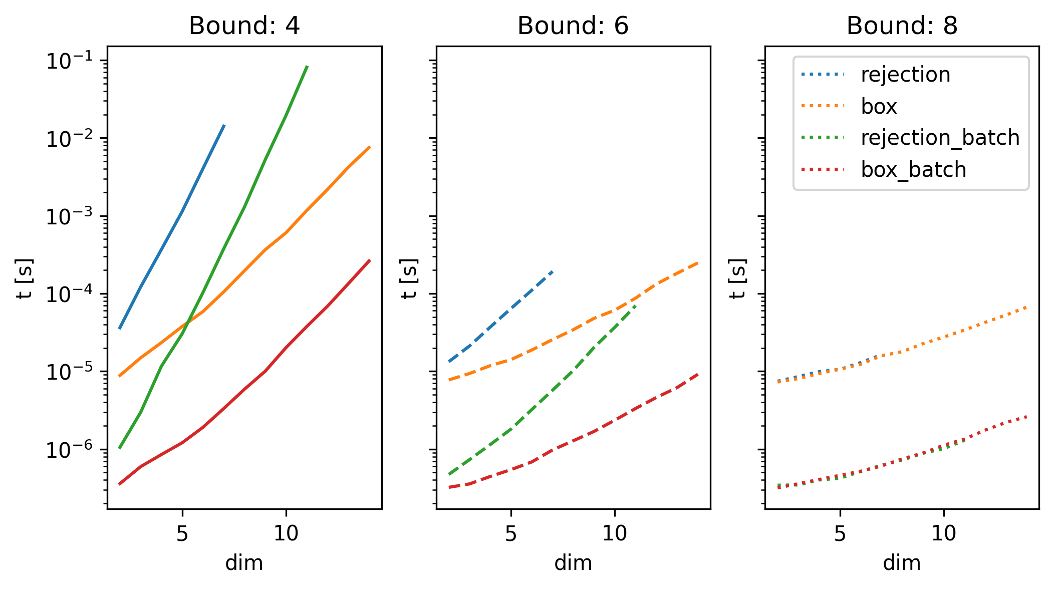
Here, we can see three things:
- batch sampling is much faster than the non-batched version
- sampling from the box constrained region first massively speeds up the sampling overall for ‘tight’ bounds
- there is a point where it does not matter which method we choose to use, since the cost is not the constraining factor anymore, but the bounds of the robot are the main constraint. However, there is alo no downside in choosing the ‘more complex’ method of sampling from the box-constrained region.
We also show a benchmarking comparison, where we keep the dimension fixed (at 6), and vary the bound \(c_b\) to see how much influence this has.
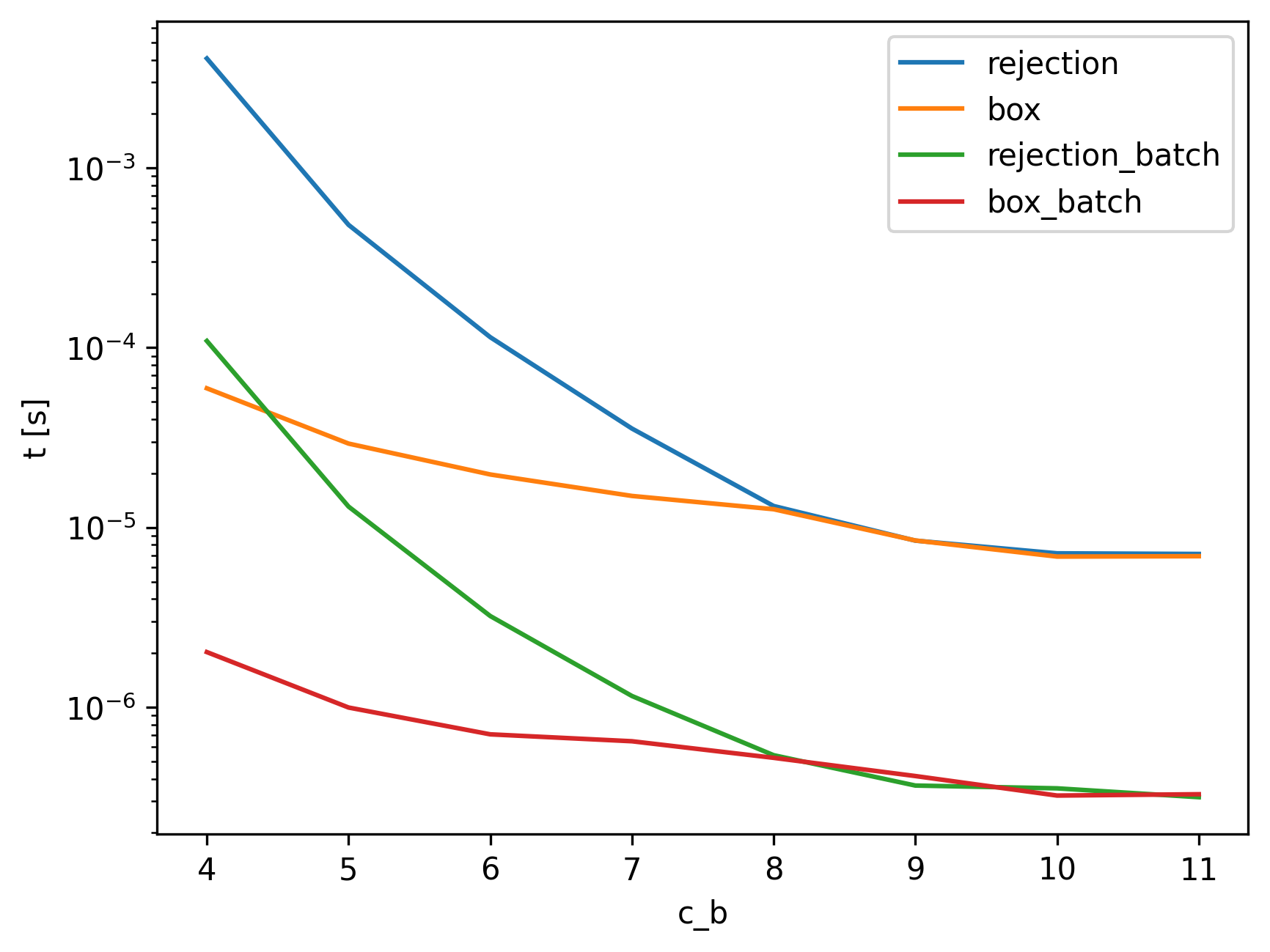
This is not that surprising once we think about the volumes of the spaces that we are sampling. Particularly, the smaller the bound, the smaller the volume of the valid region, which corresponds directly to the likelihood of sampling from it.
Takeways
It seems worth a lot to try to decrease the size of the space from which we sample by first sampling from the box-constrained region. This seems to be the case particularly in high dimensional spaces and tight bounds, where we get a speedup of up to a magnitude by sampling from the box constrained region first.
It is questionable how much the batch sampling carries over to C++ (I simply do not know how optimized generation of random matrices in e.g., Eigen is). If it carries over, it might be interesting to have a look at batched sampling using hit-and-run for very tight bounds.
Outlook
This post is motivated by the question of how we can efficiently uniformly sample the space defined by the intersection of the spaces
\[\frac{||x_s - x||}{t} < v_{max} \Rightarrow ||x_s - x|| - t v_{max} < 0\]and
\[||x_g - x|| - (t_f - t) v_{max} < 0.\]This is the space of possible solution-paths in space time-path planning. The approach I took so far for this problem is rejection sampling in the space defined by the robot-bounds, and then conditionally sampling the time dependent on the configuration that we sampled. This is fairly inefficient.
Replacing the uniform sampling of the robot-configuration with the box-constrained sampling already gives a solid speedup. I want to investigate if changing the time-sampling to something better helps the performance of ST-RRT*.
I am not sure how well batched samping works in this setting. This should be explored.