Uniformly sampling a n-ball. Quickly.
Path planning using Informed-RRT needs uniform random samples from an n-dimensional ball. Generating uniform random samples on such a n-ball is straightforward (and fairly efficient) for low dimensions (n<4). Getting to higher dimensions, the basic method becomes slow and inefficient. However, there are some better approaches. We first compare the speed of the approaches and then try to speed them up a bit.
The code for all the experiments in this post can be found here.
The algorithms for generating the points in this post are taken from here (where you can find a slightly more detailed explanation of the algorithms - unfortunately some of them are simply beyond any intuition). Some of the original codes contained a few small typos, which I fixed. In the following, I will go over them, compare their performance, and show a few simple approaches to speed them up. Note that while I would argue that I am fairly competent in python, I am by no means an expert. As such I am sure that most of the methods could be sped up even further if desired by implementing the underlying components in a specific manner. It would also be possible to speed up this process by simply implementing some of the code in C/C++. This is specifically not done in this post.
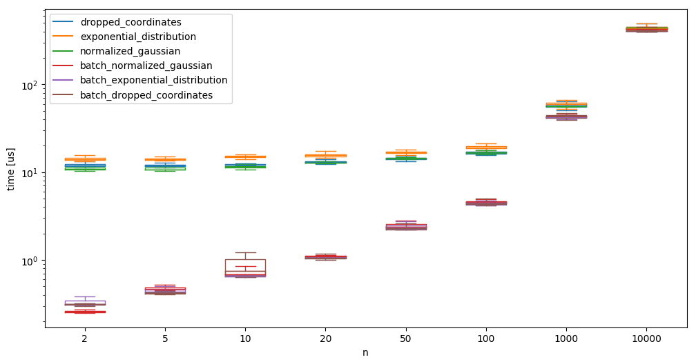
We begin with all the alorithms, look at the average time needed to generate one sample (along with outliers, etc), and check how the algorithms do on a few dimensions. We compare it agains a baseline of simply generating \(n\) uniform random numbers, and generating \(n\) normal samples (not from the multivariate gaussian, but simply \(n\) one dimensional normal samples):
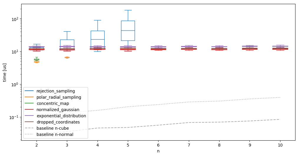
1 We can actually compute the expected percentage of accepted values as the ratio of the volume of the ball and the cube. This gives something proportional to the inverse of the Gamma function, which decays very quickly.
- Obviously visible (and mentioned in the link above as well), rejection sampling is not exacly a great idea in higher dimensions. This is mainly due to the curse of dimensionality1.
- Polar/radial sampling and concentric mapping do not have generalizations to higher dimensionalities, and are thus only usable in the low dimensional spaces.
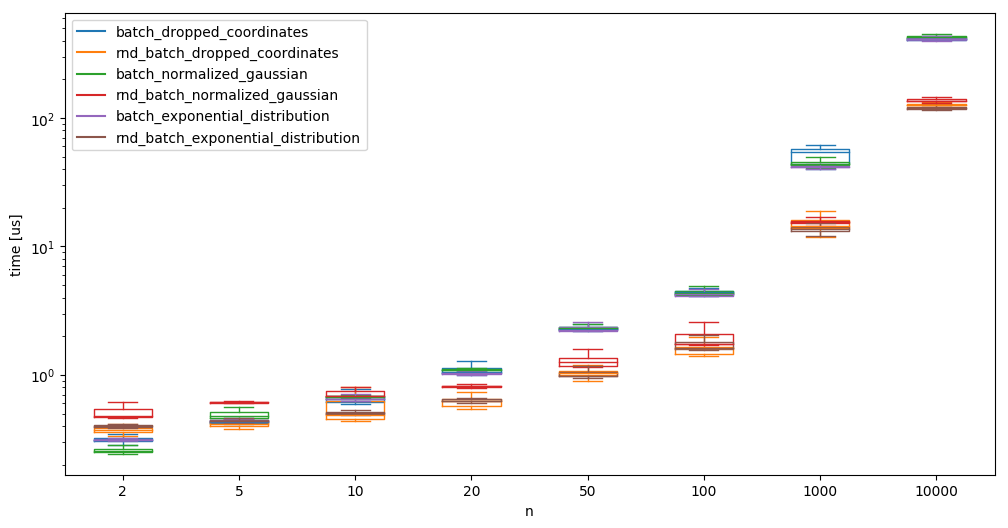
We also see that the other methods need essentially constant time, almost independent of the dimension for which we are producing the samples for low dimensions. Such a low scaling factor would be good! When running the same algorithms on much larger \(n\), the image looks different however:
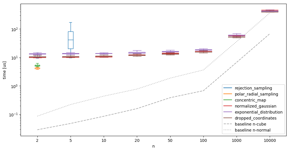
It becomes clear that the scaling is definitely not constant. We do see however, that the creation in high dimensions is comparably much more efficient: the ‘conversion’ from a n-normal sample to a n-sphere takes relatively less time - as such, it might make sense to batch the generation of the random samples. It is also interesting that the ‘normalized gaussian’ goes from the fastest (at \(n=10\)) of the high-dimensional algorithms to the slowest (at \(n=10000\)).
First we profile a run to see where the most time is spent, i.e. where we can speed up the generation the most. As an example, we have a look at the dropped_coordinates method:
1
2
3
4
5
6
7
8
9
10
11
12
13
14
15
16
17
18
19
20
21
22
         1300004 function calls in 1.837 seconds

   Ordered by: internal time

   ncalls  tottime  percall  cumtime  percall filename:lineno(function)
   100000    0.543    0.000    0.543    0.000 {method 'randn' of 'numpy.random.mtrand.RandomState' objects}
   100000    0.402    0.000    0.787    0.000 linalg.py:2325(norm)
   100000    0.317    0.000    1.782    0.000 main.py:105(dropped_coordinates)
   100000    0.286    0.000    0.286    0.000 {method 'reduce' of 'numpy.ufunc' objects}
   100000    0.070    0.000    0.921    0.000 <__array_function__ internals>:2(norm)
        1    0.056    0.056    1.837    1.837 main.py:309(test)
   100000    0.053    0.000    0.840    0.000 {built-in method numpy.core._multiarray_umath.implement_array_function}
   100000    0.041    0.000    0.053    0.000 _asarray.py:16(asarray)
   100000    0.015    0.000    0.015    0.000 {method 'conj' of 'numpy.ndarray' objects}
   100000    0.013    0.000    0.013    0.000 {built-in method builtins.isinstance}
   100000    0.012    0.000    0.012    0.000 {built-in method numpy.array}
   100000    0.012    0.000    0.012    0.000 {built-in method builtins.issubclass}
   100000    0.011    0.000    0.011    0.000 linalg.py:2321(_norm_dispatcher)
   100000    0.007    0.000    0.007    0.000 {built-in method builtins.len}
        1    0.000    0.000    1.837    1.837 {built-in method builtins.exec}
        1    0.000    0.000    1.837    1.837 <string>:1(<module>)
        1    0.000    0.000    0.000    0.000 {method 'disable' of '_lsprof.Profiler' objects}
Now, I hoped for more granularity in the profiler run for the creation of the random numbers, but for now, we take what we get. This shows that about 30% of the time in the function is spent in the creation of the random numbers, and that taking the norm occupies around 50% of the time.
How do we speed up the computation of the norm? One possibility is to attempt to implement a few things ourselves by applying domain knowledge about our numbers we are norming - e.g. no overflow can occur, so we can compute the norm naively, making the common (safe) method unnecesary. However, we would sacrifice all optimizations from numpy such as vecorization when batching the sampling, and a few other things at the numerical core of numpy. Another approach would be casting the double from randn down to a float in the hope of speeding the computation up. We leave that comparison for later.
That leaves the creation of the random samples. How do we speed that up? The first step would be profiling it - however, since the random number generator is implemented as a c-module, this is not possible.
Interlude: A very brief discourse on random number generation in numpy: In numpy random number generation is handled in two steps: A
bit_generatorproduces random bit sequences (e.g. using a version of the mersenne twister algorithm), which are then converted into the various distributions by agenerator(e.g. using the box-muller transform to obtain normally distributed numbers, or using the ziggurat algorithm for a variety of distributions).Hence, there are a few ways to speed the process up:
- Speed up
bit_generator,- Generate a shorter sequence, i.e. a different data type in the bit generator,
- Speed up the transformation into the sample from a distribution.
It turns out (unsurprisingly) that there is a library that implements all of these things already: randomgen, which is partially integrated into numpy already.
We are after the part that is not (yet) adopted: faster bit generators, faster generators, and the possibility to produce random numbers in different dtypes. Randomgen’s own performance comparison claim it is up to 10 times as fast as numpy (v1.16 - I am using v1.17 here, so that comparison is unlikely to hold).
Let’s switch the random number generator and look at the profiler output:
1
2
3
4
5
6
7
8
9
10
11
12
13
14
15
16
17
18
19
20
21
22
23
24
25
26
         2000004 function calls in 3.409 seconds

   Ordered by: internal time

   ncalls  tottime  percall  cumtime  percall filename:lineno(function)
   100000    1.230    0.000    1.678    0.000 {method 'randn' of 'randomgen.generator.Generator' objects}
   100000    0.536    0.000    1.085    0.000 linalg.py:2325(norm)
   100000    0.421    0.000    0.421    0.000 {method 'reduce' of 'numpy.ufunc' objects}
   100000    0.412    0.000    3.334    0.000 main.py:105(dropped_coordinates)
   100000    0.130    0.000    0.448    0.000 _dtype.py:319(_name_get)
   400000    0.127    0.000    0.127    0.000 {built-in method builtins.issubclass}
   200000    0.111    0.000    0.220    0.000 numerictypes.py:293(issubclass_)
   100000    0.089    0.000    0.318    0.000 numerictypes.py:365(issubdtype)
   100000    0.081    0.000    1.244    0.000 <__array_function__ internals>:2(norm)
        1    0.075    0.075    3.409    3.409 main.py:309(test)
   100000    0.065    0.000    1.151    0.000 {built-in method numpy.core._multiarray_umath.implement_array_function}
   100000    0.048    0.000    0.067    0.000 _asarray.py:16(asarray)
   100000    0.023    0.000    0.023    0.000 {method 'conj' of 'numpy.ndarray' objects}
   100000    0.018    0.000    0.018    0.000 {built-in method numpy.array}
   100000    0.014    0.000    0.014    0.000 {built-in method builtins.isinstance}
   100000    0.014    0.000    0.014    0.000 {built-in method builtins.len}
   100000    0.013    0.000    0.013    0.000 linalg.py:2321(_norm_dispatcher)
        1    0.000    0.000    3.409    3.409 {built-in method builtins.exec}
        1    0.000    0.000    3.409    3.409 <string>:1(<module>)
        1    0.000    0.000    0.000    0.000 {method 'disable' of '_lsprof.Profiler' objects}
This shows that it takes alomst twice as long! We plot it against numpy’s random sample generator for various dimensions:
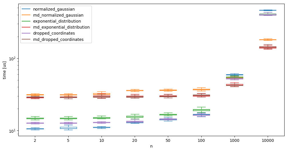
We see that while a low number of random samples is slower when using randomgen, generating high dimensional samples is much faster using randomgen.
While not always desirable/possible, we next check the possibility to generate random samples as floats rather than doubles in the hope that it speeds up some things. Note that this speedup might not be mainly due to the random number generation (although it should cut the necessary time to create the word in half), but it should also speedup the other operations for the creation of the samples (i.e. norms, mutliplications, etc);
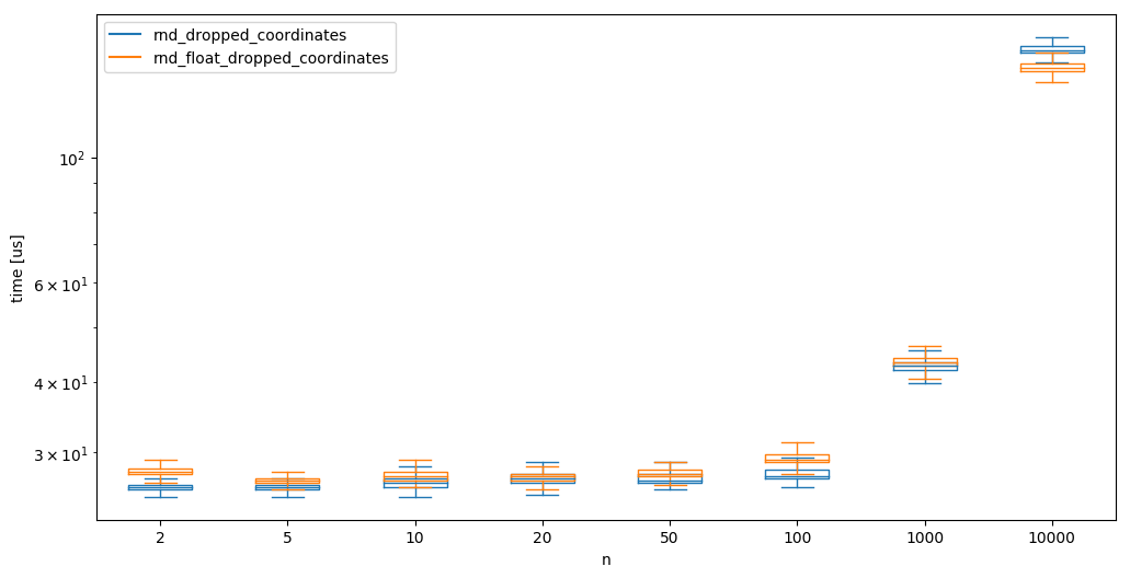
We can see that creating floats seems slightly quicker than using doubles at high dimensions, but generally, there is no notable difference.
Batching
We implement batch versions of the algorithms that work on high dimensions and run tests with a batchsize of b=100. The reported time here is the time needed to generate one sample - meaning that the time for the batch-versions is the time for a function call divided by b:
And compare randomgen with np.random again:
where we see again that randomgen takes the upper hand at a larger number of samples. This larger number is now reached quicker, as we are generating \(b\times n\) samples at a time.
Batching the creation of the random samples is obviously not always possible, as we sometimes simply do not know how many samples we need - however the speedup might be large enough (up to almost a factor 20 compared to what we started with), to allow creating too many samples (sometimes).
We’ll briefly assume that we always know many samples we need and check - is there an ‘optimal’ batch size for this case? Can we create all samples in one go, or will we encounter other issues? Obviously, at some point we are going to run into memory issues, and we are not able to produce all samples in one go anymore, But is anything going to happen before? We test dropped_coordinates (with randomgen):
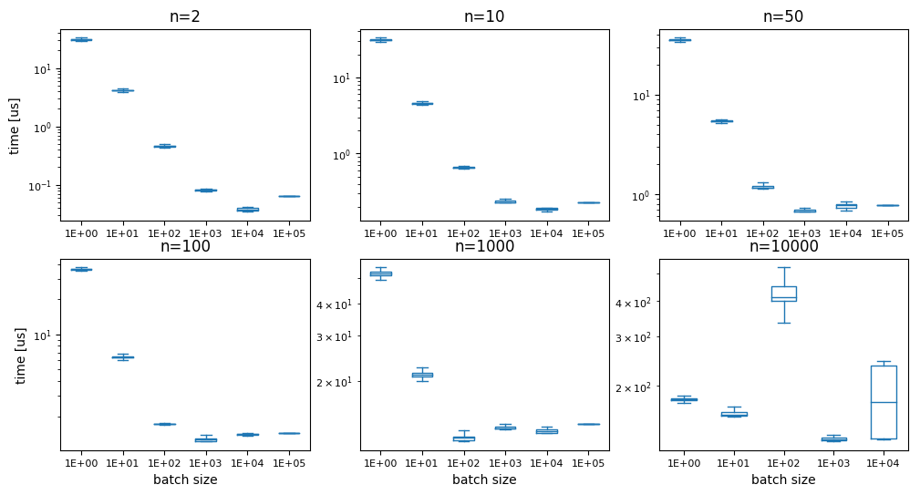
While the last graph is all over the place (and the batch size 1e5 returned a memory error), the other show a fairly consistent image: the ideal number of random samples to generate is about 10000. This manifests in the fastest time always being around the point where this number of samples was generated in one go. A possible reason for the generation to become slower again at larger sizes are likely the memory requirements and/or cache sizes. I didnt’ feel like further investigating at this point.
Conclusion/Discussion/Disclaimer
We managed to reduce the time needed to create one sample down by almost a factor of 100. This was mainly achieved by batching and usage of a better library. Note that the most important part is the choice of the algorithm though - if we would have chosen rejection sampling for the creation of the samples, we would not have had a chance to get anywhere near the performance we achieved by optimizing a ‘good’ algorithm. It is also important to take note of the fact that all of this optimization of the needed time is measured in microseconds, i.e. (depending on your application and use of the samples) probably nothing that matters too much in the grand scheme of things.
For the use that I originally had in mind (sampling from an hyperellipsoid in the Informed RRT*-algorithm), everyhing else is orders of magnitudes slower. So keep in mind that you can only optimize away what is there in the beginning - removing 100% of 20 microseconds still saves less time than getting rid of 5% of an operation that takes a second.